
(R Tutorials for Business Analyst)
R Dplyr Tutorial: Data Manipulation(Join) & Cleaning(Spread)
Introduction to Data Analysis
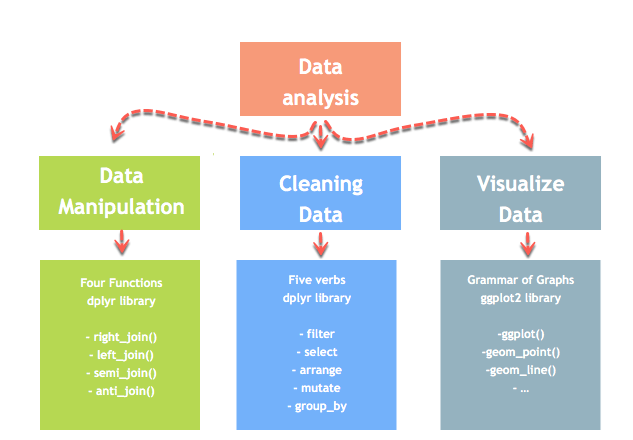
Data analysis can be divided into three parts
- Extraction: First, we need to collect the data from many sources and combine them.
- Transform: This step involves the data manipulation. Once we have consolidated all the sources of data, we can begin to clean the data.
- Visualize: The last move is to visualize our data to check irregularity.
One of the most significant challenges faced by data scientist is the data manipulation. Data is never available in the desired format. The data scientist needs to spend at least half of his time, cleaning and manipulating the data. That is one of the most critical assignments in the job. If the data manipulation process is not complete, precise and rigorous, the model will not perform correctly.
R has a library called dplyr to help in data transformation.
The dplyr library is fundamentally created around four functions to manipulate the data and five verbs to clean the data. After that, we can use the ggplot library to analyze and visualize the data.
In this tutorial, you will learn
- Data Analysis
- Merge with dplyr()
- left_join()
- right_join()
- inner_join()
- full_join()
- Multiple keys
- Data Cleaning functions
- gather()
- spread()
- separate()
- unite()
Merge with dplyr()
dplyr provides a nice and convenient way to combine datasets. We may have many sources of input data, and at some point, we need to combine them. A join with dplyr adds variables to the right of the original dataset. The beauty is dplyr is that it handles four types of joins similar to SQL
- Left_join()
- right_join()
- inner_join()
- full_join()
We will study all the joins types via an easy example.
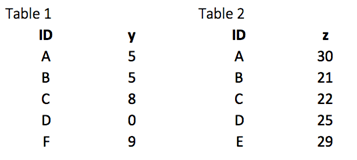
First of all, we build two datasets. Table 1 contains two variables, ID, and y, whereas Table 2 gathers ID and z. In each situation, we need to have a key-pair variable. In our case, ID is our key variable. The function will look for identical values in both tables and bind the returning values to the right of table 1.
library(dplyr)
df_primary <- tribble(
  ~ID, ~y,
   "A", 5,
   "B", 5,
   "C", 8,
   "D", 0,
  "F", 9)
df_secondary <- tribble(
  ~ID, ~y,
   "A", 30,
   "B", 21,
   "C", 22,
   "D", 25,
   "E", 29)
left_join()
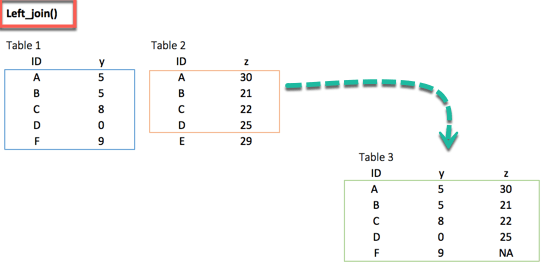
The most common way to merge two datasets is to use the left_join() function. We can see from the picture below that the key-pair matches perfectly the rows A, B, C and D from both datasets. However, E and F are left over. How do we treat these two observations? With the left_join(), we will keep all the variables in the original table and don’t consider the variables that do not have a key-paired in the destination table. In our example, the variable E does not exist in table 1. Therefore, the row will be dropped. The variable F comes from the origin table; it will be kept after the left_join() and return NA in the column z. The figure below reproduces what will happen with a left_join().
left_join(df_primary, df_secondary, by ='ID')
Output:
##
# A tibble: 5 x 3
##      ID   y.x   y.y
##   <chr> <dbl> <dbl>
## 1     A     5    30
## 2     B     5    21
## 3     C     8    22
## 4     D     0    25
## 5     F     9    NA
right_join()
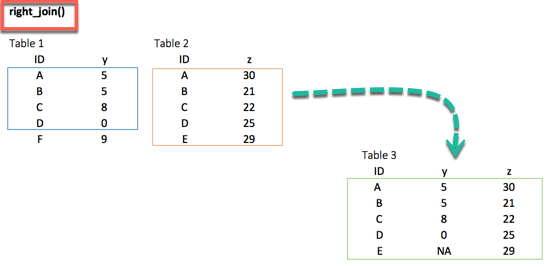
The right_join() function works exactly like left_join(). The only difference is the row dropped. The value E, available in the destination data frame, exists in the new table and takes the value NA for the column y.
right_join(df_primary, df_secondary, by = 'ID')
Output:
##
# A tibble: 5 x 3
##      ID   y.x   y.y
##   <chr> <dbl> <dbl>
## 1     A     5    30
## 2     B     5    21
## 3     C     8    22
## 4     D     0    25
## 5     E    NA    29
inner_join()
When we are 100% sure that the two datasets won’t match, we can consider to return only rows existing in both dataset. This is possible when we need a clean dataset or when we don’t want to impute missing values with the mean or median.
The inner_join()comes to help. This function excludes the unmatched rows.
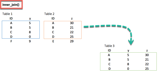
inner_join(df_primary, df_secondary, by ='ID')
output:
##
# A tibble: 4 x 3
##      ID   y.x   y.y
##   <chr> <dbl> <dbl>
## 1     A     5    30
## 2     B     5    21
## 3     C     8    22
## 4     D     0    25
full_join()
Finally, the full_join() function keeps all observations and replace missing values with NA.
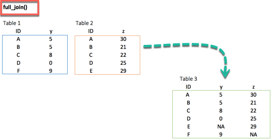
full_join(df_primary, df_secondary, by = 'ID')
Output:
## # A tibble: 6 x 3
##      ID   y.x   y.y
##   <chr> <dbl> <dbl>
## 1     A     5    30
## 2     B     5    21
## 3     C     8    22
## 4     D     0    25
## 5     F     9    NA
## 6     E    NA    29
Multiple keys pairs
Last but not least, we can have multiple keys in our dataset. Consider the following dataset where we have years or a list of products bought by the customer.
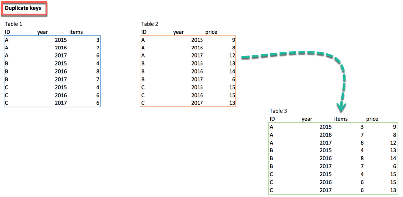
If we try to merge both tables, R throws an error. To remedy the situation, we can pass two key-pairs variables. That is, ID and year which appear in both datasets. We can use the following code to merge table1 and table 2
df_primary <- tribble(
  ~ID, ~year, ~items,
  "A", 2015,3,
  "A", 2016,7,
  "A", 2017,6,
  "B", 2015,4,
  "B", 2016,8,
  "B", 2017,7,
  "C", 2015,4,
  "C", 2016,6,
  "C", 2017,6)
df_secondary <- tribble(
  ~ID, ~year, ~prices,
  "A", 2015,9,
  "A", 2016,8,
  "A", 2017,12,
  "B", 2015,13,
  "B", 2016,14,
  "B", 2017,6,
  "C", 2015,15,
  "C", 2016,15,
  "C", 2017,13)
left_join(df_primary, df_secondary, by = c('ID', 'year'))
Output:
## # A tibble: 9 x 4
##      ID  year items prices
##   <chr> <dbl> <dbl>  <dbl>
## 1     A  2015     3      9
## 2     A  2016     7      8
## 3     A  2017     6     12
## 4     B  2015     4     13
## 5     B  2016     8     14
## 6     B  2017     7      6
## 7     C  2015     4     15
## 8     C  2016     6     15
## 9     C  2017     6     13
Data Cleaning functions
Following are four important functions to tidy the data:
- gather(): Transform the data from wide to long
- spread(): Transform the data from long to wide
- separate(): Split one variable into two
- unit(): Unit two variables into one
We use the tidyr library. This library belongs to the collection of the library to manipulate, clean and visualize the data. If we install R with anaconda, the library is already installed. We can find the library here, https://anaconda.org/r/r-tidyr.
If not installed already, enter the following command
install tidyr : install.packages(“tidyr”)
to install tidyr
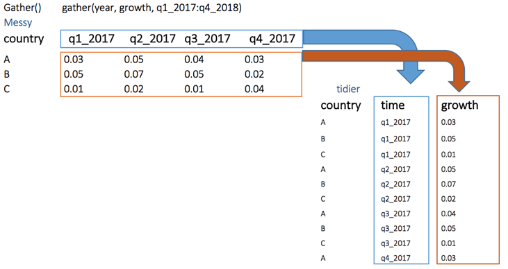
gather()
The objectives of the gather() function is to transform the data from wide to long.
gather(data, key, value, na.rm = FALSE)
Arguments:
-data: The data frame used to reshape the dataset
-key: Name of the new column created
-value: Select the columns used to fill the key column
-na.rm: Remove missing values. FALSE by default
Below, we can visualize the concept of reshaping wide to long. We want to create a single column named growth, filled by the rows of the quarter variables.
library(tidyr)
# Create a messy dataset
messy <- data.frame(
  country = c("A", "B", "C"),
  q1_2017 = c(0.03, 0.05, 0.01),
  q2_2017 = c(0.05, 0.07, 0.02),
  q3_2017 = c(0.04, 0.05, 0.01),
  q4_2017 = c(0.03, 0.02, 0.04))
messy
Output:
##   country q1_2017 q2_2017 q3_2017 q4_2017
## 1       A    0.03    0.05    0.04    0.03
## 2       B    0.05    0.07    0.05    0.02
## 3       C    0.01    0.02    0.01    0.04
# Reshape the data
tidier <-messy %>%
gather(quarter, growth, q1_2017:q4_2017)
tidier
Output:
##    country quarter growth
## 1        A q1_2017   0.03
## 2        B q1_2017   0.05
## 3        C q1_2017   0.01
## 4        A q2_2017   0.05
## 5        B q2_2017   0.07
## 6        C q2_2017   0.02
## 7        A q3_2017   0.04
## 8        B q3_2017   0.05
## 9        C q3_2017   0.01
## 10       A q4_2017   0.03
## 11       B q4_2017   0.02
## 12       C q4_2017   0.04
In the gather() function, we create two new variable quarter and growth because our original dataset has one group variable: i.e. country and the key-value pairs.
spread()
The spread() function does the opposite of gather.
spread(data, key, value)
arguments:
- data: The data frame used to reshape the dataset
- key: Column to reshape long to wide
- value: Rows used to fill the new column
We can reshape the tidier dataset back to messy with spread()
# Reshape the data
messy_1 <- tidier %>%
  spread(quarter, growth)
messy_1
Output:
##   country q1_2017 q2_2017 q3_2017 q4_2017
## 1       A    0.03    0.05    0.04    0.03
## 2       B    0.05    0.07    0.05    0.02
## 3       C    0.01    0.02    0.01    0.04
separate()
The separate() function splits a column into two according to a separator. This function is helpful in some situations where the variable is a date. Our analysis can require focussing on month and year and we want to separate the column into two new variables.
Syntax:
separate(data, col, into, sep= "", remove = TRUE)
arguments:
-data: The data frame used to reshape the dataset
-col: The column to split
-into: The name of the new variables
-sep: Indicates the symbol used that separates the variable, i.e.:  "-", "_", "&"
-remove: Remove the old column. By default sets to TRUE.
We can split the quarter from the year in the tidier dataset by applying the separate() function.
separate_tidier <-tidier %>%
separate(quarter, c("Qrt", "year"), sep ="_")
head(separate_tidier)
Output:
##   country Qrt year growth
## 1       A  q1 2017   0.03
## 2       B  q1 2017   0.05
## 3       C  q1 2017   0.01
## 4       A  q2 2017   0.05
## 5       B  q2 2017   0.07
## 6       C  q2 2017   0.02
unite()
The unite() function concanates two columns into one.
Syntax:
unit(data, col, conc ,sep= "", remove = TRUE)
arguments:
-data: The data frame used to reshape the dataset
-col: Name of the new column
-conc: Name of the columns to concatenate
-sep: Indicates the symbol used that unites the variable, i.e:  "-", "_", "&"
-remove: Remove the old columns. By default, sets to TRUE
In the above example, we separated quarter from year. What if we want to merge them. We use the following code:
unit_tidier <- separate_tidier %>%
  unite(Quarter, Qrt, year, sep ="_")
head(unit_tidier)
output:
##   country Quarter growth
## 1       A q1_2017   0.03
## 2       B q1_2017   0.05
## 3       C q1_2017   0.01
## 4       A q2_2017   0.05
## 5       B q2_2017   0.07
## 6       C q2_2017   0.02
Summary
Following are four important functions used in dplyr to merge two datasets.
| Function | Objectives | Arguments | Multiple keys |
|---|---|---|---|
| left_join() | Merge two datasets. Keep all observations from the origin table | data, origin, destination, by = “ID” | origin, destination, by = c(“ID”, “ID2”) |
| right_join() | Merge two datasets. Keep all observations from the destination table | data, origin, destination, by = “ID” | origin, destination, by = c(“ID”, “ID2”) |
| inner_join() | Merge two datasets. Excludes all unmatched rows | data, origin, destination, by = “ID” | origin, destination, by = c(“ID”, “ID2”) |
| full_join() | Merge two datasets. Keeps all observations | data, origin, destination, by = “ID” | origin, destination, by = c(“ID”, “ID2”) |
Using the tidyr Library you can transform a dataset with the gather(), spread(), separate() and unit() functions.
| Function | Objectives | Arguments |
|---|---|---|
| gather() | Transform the data from wide to long | (data, key, value, na.rm = FALSE) |
| spread() | Transform the data from long to wide | (data, key, value) |
| separate() | Split one variables into two | (data, col, into, sep= “”, remove = TRUE) |
| unit() | Unit two variables into one | (data, col, conc ,sep= “”, remove = TRUE) |
Disclaimer: The information and code presented within this recipe/tutorial is only for educational and coaching purposes for beginners and developers. Anyone can practice and apply the recipe/tutorial presented here, but the reader is taking full responsibility for his/her actions. The author (content curator) of this recipe (code / program) has made every effort to ensure the accuracy of the information was correct at time of publication. The author (content curator) does not assume and hereby disclaims any liability to any party for any loss, damage, or disruption caused by errors or omissions, whether such errors or omissions result from accident, negligence, or any other cause. The information presented here could also be found in public knowledge domains.
Learn by Coding: v-Tutorials on Applied Machine Learning and Data Science for Beginners
Latest end-to-end Learn by Coding Projects (Jupyter Notebooks) in Python and R:
All Notebooks in One Bundle: Data Science Recipes and Examples in Python & R.
End-to-End Python Machine Learning Recipes & Examples.
End-to-End R Machine Learning Recipes & Examples.
Applied Statistics with R for Beginners and Business Professionals
Data Science and Machine Learning Projects in Python: Tabular Data Analytics
Data Science and Machine Learning Projects in R: Tabular Data Analytics
Python Machine Learning & Data Science Recipes: Learn by Coding
R Machine Learning & Data Science Recipes: Learn by Coding
Comparing Different Machine Learning Algorithms in Python for Classification (FREE)
There are 2000+ End-to-End Python & R Notebooks are available to build Professional Portfolio as a Data Scientist and/or Machine Learning Specialist. All Notebooks are only $29.95. We would like to request you to have a look at the website for FREE the end-to-end notebooks, and then decide whether you would like to purchase or not.
R tutorials for Business Analyst – R Data Frame Sorting using Order()
Pandas Example – Write a Pandas program to merge two given dataframes with different columns