
(R Tutorials for Citizen Data Scientist)
Statistics with R for Business Analysts – Time Series Analysis
Time series is a series of data points in which each data point is associated with a timestamp. A simple example is the price of a stock in the stock market at different points of time on a given day. Another example is the amount of rainfall in a region at different months of the year. R language uses many functions to create, manipulate and plot the time series data. The data for the time series is stored in an R object called time-series object. It is also a R data object like a vector or data frame.
The time series object is created by using the ts() function.
Syntax
The basic syntax for ts() function in time series analysis is −
timeseries.object.name <- ts(data, start, end, frequency)
Following is the description of the parameters used −
- data is a vector or matrix containing the values used in the time series.
- start specifies the start time for the first observation in time series.
- end specifies the end time for the last observation in time series.
- frequency specifies the number of observations per unit time.
Except the parameter “data” all other parameters are optional.
Example
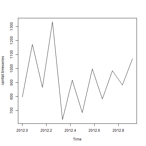
Consider the annual rainfall details at a place starting from January 2012. We create an R time series object for a period of 12 months and plot it.
# Get the data points in form of a R vector.
rainfall <- c(799,1174.8,865.1,1334.6,635.4,918.5,685.5,998.6,784.2,985,882.8,1071)

# Convert it to a time series object.
rainfall.timeseries <- ts(rainfall,start = c(2012,1),frequency = 12)

# Print the timeseries data.
print(rainfall.timeseries)

# Give the chart file a name.
png(file = "rainfall.png")

# Plot a graph of the time series.
plot(rainfall.timeseries)

# Save the file.
dev.off()
When we execute the above code, it produces the following result and chart −
Jan    Feb    Mar    Apr    May     Jun    Jul    Aug    Sep
2012  799.0  1174.8  865.1  1334.6  635.4  918.5  685.5  998.6  784.2
        Oct    Nov    Dec
2012  985.0  882.8 1071.0
The Time series chart −
Different Time Intervals
The value of the frequency parameter in the ts() function decides the time intervals at which the data points are measured. A value of 12 indicates that the time series is for 12 months. Other values and its meaning is as below −
- frequency = 12 pegs the data points for every month of a year.
- frequency = 4 pegs the data points for every quarter of a year.
- frequency = 6 pegs the data points for every 10 minutes of an hour.
- frequency = 24*6 pegs the data points for every 10 minutes of a day.
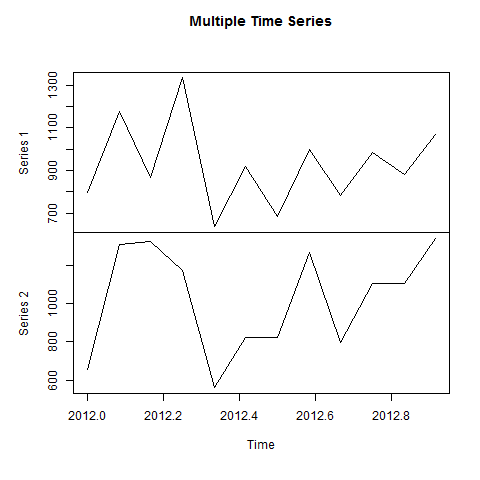
Multiple Time Series
We can plot multiple time series in one chart by combining both the series into a matrix.
# Get the data points in form of a R vector.
rainfall1 <- c(799,1174.8,865.1,1334.6,635.4,918.5,685.5,998.6,784.2,985,882.8,1071)
rainfall2 <-
           c(655,1306.9,1323.4,1172.2,562.2,824,822.4,1265.5,799.6,1105.6,1106.7,1337.8)

# Convert them to a matrix.
combined.rainfall <-  matrix(c(rainfall1,rainfall2),nrow = 12)

# Convert it to a time series object.
rainfall.timeseries <- ts(combined.rainfall,start = c(2012,1),frequency = 12)

# Print the timeseries data.
print(rainfall.timeseries)

# Give the chart file a name.
png(file = "rainfall_combined.png")

# Plot a graph of the time series.
plot(rainfall.timeseries, main = "Multiple Time Series")

# Save the file.
dev.off()
When we execute the above code, it produces the following result and chart −
           Series 1  Series 2
Jan 2012    799.0    655.0
Feb 2012   1174.8   1306.9
Mar 2012    865.1   1323.4
Apr 2012   1334.6   1172.2
May 2012    635.4    562.2
Jun 2012    918.5    824.0
Jul 2012    685.5    822.4
Aug 2012    998.6   1265.5
Sep 2012    784.2    799.6
Oct 2012    985.0   1105.6
Nov 2012    882.8   1106.7
Dec 2012   1071.0   1337.8
The Multiple Time series chart −
Time Series Analysis in R using Neural Networks | Data Science with R
Statistics with R for Business Analysts – Time Series Analysis
Disclaimer: The information and code presented within this recipe/tutorial is only for educational and coaching purposes for beginners and developers. Anyone can practice and apply the recipe/tutorial presented here, but the reader is taking full responsibility for his/her actions. The author (content curator) of this recipe (code / program) has made every effort to ensure the accuracy of the information was correct at time of publication. The author (content curator) does not assume and hereby disclaims any liability to any party for any loss, damage, or disruption caused by errors or omissions, whether such errors or omissions result from accident, negligence, or any other cause. The information presented here could also be found in public knowledge domains.
Learn by Coding: v-Tutorials on Applied Machine Learning and Data Science for Beginners
Latest end-to-end Learn by Coding Projects (Jupyter Notebooks) in Python and R:
All Notebooks in One Bundle: Data Science Recipes and Examples in Python & R.
End-to-End Python Machine Learning Recipes & Examples.
End-to-End R Machine Learning Recipes & Examples.
Applied Statistics with R for Beginners and Business Professionals
Data Science and Machine Learning Projects in Python: Tabular Data Analytics
Data Science and Machine Learning Projects in R: Tabular Data Analytics
Python Machine Learning & Data Science Recipes: Learn by Coding
R Machine Learning & Data Science Recipes: Learn by Coding
Comparing Different Machine Learning Algorithms in Python for Classification (FREE)
There are 2000+ End-to-End Python & R Notebooks are available to build Professional Portfolio as a Data Scientist and/or Machine Learning Specialist. All Notebooks are only $29.95. We would like to request you to have a look at the website for FREE the end-to-end notebooks, and then decide whether you would like to purchase or not.