It is often useful to create a model using simulation. Usually, this takes the form of generating a series of random observations (often based on a specific statistical distribution) and then studying the resulting observations using techniques described throughout the rest of this website. This approach is commonly called Monte Carlo simulation.

Excel Function: Excel provides two functions for generating random numbers

RAND() – generates a random number between 0 and 1

RANDBETWEEN(a, b) – generates a random integer between a and b

Note that these functions are volatile, in the sense that every time there is a change to the worksheet their value is recalculated and a different random number is generated. If you don’t want this to happen, then enter RAND() on the formula bar and press the function key F9. This will replace the formula RAND() by the value generated. Alternatively, you can copy the random number (or a range of random numbers) using Ctrl-C and then paste them back into the same location using Home > Clipboard|Paste and then selecting the Paste Values option.

RANDBETWEEN only generates integer values. If you want a random number which could be any decimal number between a and b, then use the following formula instead:

= a +(b − a) * RAND()

Excel 365 Function: Excel 365 provides the following dynamic array function with spillover.

RANDARRAY(nrows, ncols, a, b): fills an nrows × ncols range starting in the current cell with random numbers between a and b inclusive.

RANDARRAY(nrows, ncols, a, b, TRUE): fills an nrows × ncols range starting in the current cell with random integers between a and b inclusive.

If omitted nrows, ncols and b default to 1 and a defaults to 0.

E.g. to generate 10 random numbers between 0 and 1 using Excel 365, you enter the formula =RANDARRAY(10) in cell A1 and press Enter.

If you are not using Excel 365, you can instead enter the formula =RAND() in cell A1, highlight range A1:A10 and press Ctrl-D.

Real Statistics Function: The Real Statistics Resource Pack provides the RANDOM function which generates a non-volatile random number.

RANDOM(a, b, FALSE, seed) = random number between a and b; i.e a non-volatile version of a + (b − a) * RAND()

RANDOM(a, b, TRUE, seed) = random integer between a and b, inclusive; i.e. a non-volatile version of RANDBETWEEN(a, b)

If a is omitted it defaults to 0, if b is omitted it defaults to 1 and if the third argument is omitted it defaults to FALSE.

If seed ≤ 0 or omitted then no seed is used, while if it is a positive value, then this value is used as a seed. A seed can be used to generate a repeatable sequence of pseudo-random values.

Random numbers based on a distribution

Excel Data Analysis Tool: In addition to the RAND and RANDBETWEEN functions, Excel provides the Random Number Generation data analysis tool which generates random numbers in the form of a table that adheres to one of several distributions. You can specify the following values with this tool:

Number of Variables = number of samples. This is the number of columns in the output table generated by Excel.

Number of Random Numbers = the size of each sample. This is the number of rows in the output table generated by Excel.

Distribution desired: specifies one of the following distributions:

• Uniform, specify α (lower bound) and β (upper bound)
• Normal, specify µ (mean) and σ (standard deviation)
• Bernoulli, specify p (probability of success); like the binomial distribution with n = 1
• Binomial, specify p (probability of success) and n (number of trials)
• Poisson, specify λ (mean)
• Patterned – specify a lower and upper bound, a step, repetition rate for values, and repetition rate for the sequence
• Discrete – specify a value and the associated probability range. The range must contain two columns: the left column contains values and the right column contains probabilities associated with the value in that row. The sum of the probabilities must be 1.

Random Seed = an optional value used to generate the first random number. You can reuse this value later to ensure that the same random numbers are produced. If left blank a new random number will be generated each time.

Example 1: Simulate the Central Limit Theorem by generating 100 samples of size 50 from a population with a uniform distribution in the interval [50, 150]. Thus each data element in each sample is a randomly selected, equally likely value between 50 and 150.

Select Data > Analysis|Data Analysis and choose the Random Number Generation data analysis tool. Fill in the dialog box that appears as shown in Figure 1.

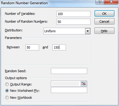
Figure 1 – Random Number Generator Dialog Box

The output is an Excel array with 50 rows and 100 columns. We then calculate the mean of each column using the AVERAGE function. The result is a row with 100 entries containing the means of each of the 100 samples. This is shown in Figure 2 (reformatted as a 10 × 10 array to fit on the screen better).

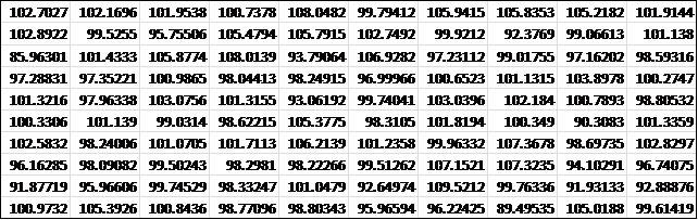
Figure 2 – Means of the 100 random samples

Using Excel’s Histogram data analysis tool we now create a histogram of the 100 sample means, as shown on the right side of Figure 3.

Figure 3 – Testing the Central Limit Theorem

The mean of the sample means is 100.0566 and the standard deviation is 4.318735. As you can see the histogram is reasonably similar to the bell-shaped curve of a normal distribution.

Since the sample was taken from a uniform distribution in the range [50, 150], as can be seen from Uniform Distribution, the population mean is  = 100 and the standard deviation is  = 28.86751.

Based on the Central Limit Theorem, we expect that the mean of the sample means will be the population mean, which seems to be the case since 100.0566 is quite close to 100. We also expect that the standard deviation of the sample means to be

which is quite close to the observed value of 4.318735.

Observation: We can also manually generate a random sample that follows any of the distributions supported by Excel without using the data analysis tool. E.g. to generate a sample of size 25 which follows a normal distribution with mean 60 and standard deviation 20, you simply use the formula =NORMINV(RAND(),60,20) 25 times.

In Figure 4 we have done just that in column C (i.e. a column of values). E.g. cell C4 contains the formula

=NORMINV(B4,$G$3,$G$4)

In column D we place the probabilities (i.e. the  values) where e.g. D4 contains the formula

=NORMDIST(C4,$G$3,$G$4,FALSE)

Finally, we create a scatter diagram of the x values vs the y values, which as you can see looks like the bell curve of the normal distribution.

Figure 4 – Creating a sample from a normal distribution

Observation: In a similar fashion we can generate random samples for any of the distributions supported by Excel (or the Real Statistics Resource Pack). E.g. to generate one element from the Poisson distribution with mean = 7, we use the formula =POISSON_INV(RAND(),7) where POISSON_INV is the Real Statistics function described in Poisson Distribution.

Weighted random numbers

When using the Excel random number formula =RANDBETWEEN(1, 4), the probability that any of the values 1, 2, 3 or 4 occurs is the identical 25%. We now describe a way of varying the probability that any specific value occurs.

Real Statistics Function: The Real Statistics Resource Pack provides the following function.

WRAND(R1) = a random integer between 1 and n where R1 is an n × 1 column range of weights.

Example 2: Generate 20 random numbers from the set {1, 2, 3, 4} using the weights in range H4:H7 of Figure 5.

Thus, the probability of generating a 1 is 50/(50+10+20+20) = 50%, the probability of generating a 2 is 10/(50+10+20+20) = 10%, etc.

The result is shown in column J of Figure 5.

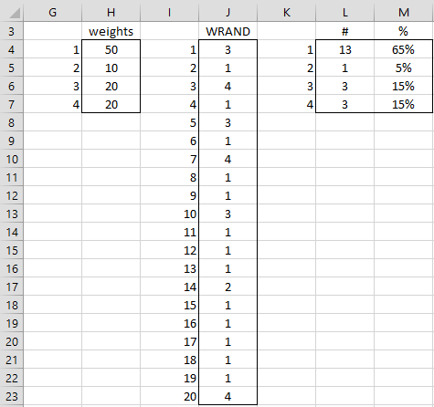
Figure 5 – Weighted random number generation

Here, each cell in range J4:J23 contains the formula =WRAND($H$4:$H$7). Range L3:M7 contains a tabulation of the number of times each of the values 1, 2, 3 and 4 occurs in the range J4:J23. As we see, the frequencies are similar (but not identical) to the probabilities which result from the weights.