The method described in Goodness of Fit can also be used to determine whether two sets of data are independent of each other. Such data are organized in what are called contingency tables, as described in Example 1. In these cases df = (row count – 1) (column count – 1).

Excel Function: The CHISQ.TEST function described in Goodness of Fit can be extended to support ranges consisting of multiple rows and columns. For R1 = the array of observed data and R2 = the array of expected values, we have

CHISQ.TEST(R1, R2) = CHISQ.DIST(x, df) where x is calculated from R1 and R2 as in Definition 2 of Goodness of Fit and df = (row count – 1) (column count – 1).

The ranges R1 and R2 must have the same size and shape and can only contain numeric values.

For versions of Excel prior to Excel 2010, the CHISQ.TEST function doesn’t exist. Instead you need to use the equivalent function, CHITEST.

Example 1: A survey is conducted of 175 young adults whose parents are classified either as wealthy, middle class or poor to determine their highest level of schooling (graduated from university, graduated from high school or neither). The results are summarized on the left side of Figure 1 (Observed Values). Based on the data collected is the person’s level of schooling independent of their parents’ wealth?

Figure 1 – Observed data and expected values for Example 1

We set the null hypothesis to be

H₀: Highest level of schooling attained is independent of parents’ wealth

We use the chi-square test, and so need to calculate the expected values that correspond to the observed values in the table above. To accomplish this we use the fact (by Definition 3 of Basic Probability Concepts) that if A and B are independent events then P(A ∩ B) = P(A) ∙ P(B). We also assume that the proportions for the sample are good estimates for the probabilities of the expected values.

We now show how to construct the table of expected values (i.e. the Expected Values in Figure 1). We know that 45 of the 175 people in the sample are from wealthy families, and so the probability that someone in the sample is from a wealthy family is 45/175 = 25.7%. Similarly the probability that someone in the sample graduated from university is 68/175 = 38.9%. But based on the null hypothesis, the event of being from a wealthy family is independent of graduating from university, and so the expected probability of both events is simply the product of the two events, or 25.7% ∙ 38.9% = 10.0%. Thus, based on the null hypothesis, we expect that 10.0% of 175 = 17.5 people are from a wealthy family and have graduated from university.

In this way we can fill out the table for expected values. We start by setting all the totals in the Expected Values table to be the same as the corresponding total in the Observed Values table (e.g. cell K6 contains the formula =E6). We then set the value of every cell in the Expected Values table to be

(row total ∙ col total) / grand total

E.g. cell H6 contains the formula =K6*H9/K9. An alternative approach for filling in all the cells in the Expected Values table is to place the following array formula in range H6:J8 (and then press Ctrl-Shft-Enter):

=MMULT(K6:K8,H9:J9)/K9

See Matrix Operations for more information about the MMULT array function. We can now calculate the p-value for the chi-square test statistic as CHITEST(Obs, Exp, df) where Obs is the 3 × 3 array of observed values, Exp = the 3 × 3 array of expected values and df = (row count – 1) (column count – 1) = 2 ∙ 2 = 4. Since

CHITEST(B6:D8,H6:J8) = 0.003273 < .05 = α

we reject the null hypothesis and conclude that the level of schooling attained is not independent of parents’ wealth.

Example 2: A researcher wants to know whether there is a significant difference in two therapies for curing patients of cocaine dependence (defined as not taking cocaine for at least 6 months). She tests 150 patients and obtains the results in the upper left part of the table below (labeled Observed Values).

Figure 2 – Chi-square tests for independence

We establish the following null hypothesis:

H₀: There is no difference between the two therapies’ ability to cure cocaine dependence

We next calculate the Expected Values from the Observed Values and then the p-value of the chi-square statistic as we did in Example 1. This time, however, we will use the approach employed in Example 2 of Goodness of Fit, namely calculating the Pearson’s chi-square test statistic directly (using Definition 2 of Goodness of Fit). The value of this statistic is 5.516 (cell D17 in Figure 2). Since we are dealing with a 2 × 2 table of observations, df = (2 – 1)(2 – 1) = 1. Finally we observe that

p-value = CHIDIST(χ², df) = CHIDIST(5.516,1) = .0188 < .05 = α

χ²-crit = CHIINV(α, df) = CHIINV(.05,1) = 3.841 < 5.516 = χ²-obs

and so we reject the null hypothesis and conclude there is a significant difference in the cure rate between the two therapies.

As was mentioned in Goodness of Fit, the maximum likelihood test is a more precise version of the chi-square test employed thus far. The lower right-hand side of the worksheet in Figure 2 shows how to calculate the maximum likelihood statistic (using Definition 1 of Goodness of Fit). The value of this statistic is 5.725, which is not much different from the test statistic we obtained using the Pearson’s test. Since this statistic is also approximately chi-square with one degree of freedom, the analysis is quite similar:

p-value = CHIDIST(χ², df) = CHIDIST(5.725,1) = .015 < .05 = α

χ²-crit = CHIINV(α, df) = CHIINV(.05,1) = 3.841 < 5.725 = χ²-obs

and so once again, we reject the null hypothesis and conclude there is significant difference in the results for the two therapies.

Observation: It is very important to include all observations in the test. E.g. if in Example 2 we only test Cured vs. Therapy 1 and 2, we will get erroneous results. We need to include Not Cured as well as Cured.

Real Statistics Excel Functions: The following supplemental functions are provided in the Real Statistics Resource Pack:

CHI_STAT2(R1, R2) = Pearson’s chi-square statistic for observation values in range R1 and expectation values in range R2

CHI_MAX2(R1, R2) = Maximum likelihood chi-square statistic for observation values in range R1 and expectation values in range R2

CHI_STAT(R1) = Pearson’s chi-square statistic for observation values in range R1. This is CHI_STAT2(R1, R2) where R2 is the expectation values calculated from R1.

CHI_MAX(R1) = Maximum likelihood chi-square statistic for observation values in range R1. This is CHI_MAX2(R1, R2) where R2 is the expectation values calculated from R1.

CHI_TEST(R1) = p-value for Pearson’s chi-square statistic for observation values in range R1. This is CHITEST(R1, R2) where R2 is the expectation values calculated from R1.

CHI_MAX_TEST(R1) = p-value for Maximum likelihood chi-square statistic for observation values in range R1

The ranges R1 and R2 must contain only numeric values.

Real Statistics Data Analysis Tool: In addition, the Real Statistics Resource Pack provides a supplemental Chi-Square Test data analysis tool. To use this tool for Example 1 enter Ctrl-m and select the Chi-square Test option. A dialog box as in Figure 3 appears.

Figure 3 – Dialog box for Chi-square Test

Insert the observation data into the Input Range (excluding the totals, but optionally including the row and column headings; i.e. range A5:D8), click on the Excel format radio button and press the OK button. Leave the Fisher Exact Test option unchecked (see Fisher Exact Test for use of this option).

The data analysis tool builds an array with the expected values and performs both the Pearson’s and maximum likelihood chi-square tests. The Cramer effect size, and for 2 × 2 contingency tables the Odds Ratio effect size, as described in Effect Size for Chi-square are also calculated. The output from the data analysis tool for the data in Example 1 in shown in Figure 4.

Figure 4 – Chi-Square data analysis tool output for Example 1

Observation: As described in Goodness of Fit, the expected frequency for any cell in the contingency table  should generally be at least 5. With small tables (especially 2 × 2 tables), cells with expected frequencies of at least 10 would be preferable.

For large contingency tables, a small percentage of cells with expected frequency of less than 5 can be acceptable. Even for smaller contingency tables having one cell with expected frequency of less than 5 may not cause big problems, but it is probably a better choice to use Fisher’s Exact Test in this case. In any event, you should avoid using the chi-square test where there is an expected frequency of less than 1 in any cell.

If the expected frequency for one or more cell is less than 5, it may be beneficial to combine one or more cells so that this condition can be met, although this must be done in such a way as to not bias the results.

Observation: In addition to the usual Excel input data format, the Real Statistics Chi Square Test data analysis tool supports another input data format called standard format. This format is similar to that used by SPSS and other statistical analysis programs.

Example 3: A survey is conducted of 38 young adults whose parents are classified either as wealthy, middle class or poor to determine whether they will graduate from university or not. The results are summarized in the table on the left side of Figure 5 (only the first 13 of 38 rows of data are shown). Based on the data collected is a person’s level of schooling independent of their parents’ wealth?

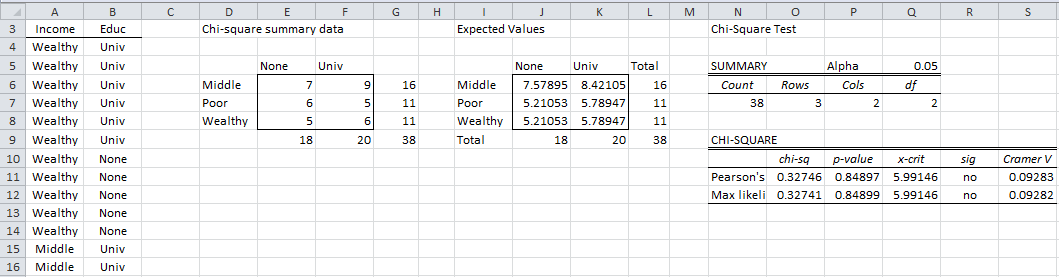
Figure 5 – Data and chi-square tests for Example 3

Once again enter Ctrl-m and select the Chi-square data analysis tool. When the dialog box shown in Figure 3 appears, insert A3:B41 into the Input Range, click on the Standard format radio button and press the OK button.

The data analysis tool first builds a contingency table (range D5:F8 of Figure 5) and performs the same type of analysis as for Example 1 and 2. Since sig = no (cells R11 and R12) we cannot reject the null hypothesis that a student’s graduating from university is independent of his/her parents’ level of income.

Observation: Example 3 uses the two column version of the standard format. There is also a three column version, which is a frequency table version of the other standard format. This is demonstrated in Figure 6 where A4:C9 is inserted in the Input Range (or A3:C9 if Column/row headings included with data is checked). The output is identical to that shown in Figure 5.

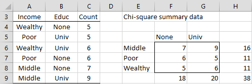
Figure 6 – Standard format