EASY IMAGE PROCESSING IN R USING THE MAGICK PACKAGE
This article describes how to perform image processing in R using the magick R package, which is binded to ImageMagick library: the most comprehensive open-source image processing library available.
The magick R package supports:
- Many common formats: png, jpeg, tiff, pdf, etc
- Different manipulations types: rotate, scale, crop, trim, flip, blur, etc.
All operations are vectorized using the Magick++ STL meaning they operate either on a single frame or a series of frames for working with layers, collages, or animation.
In RStudio images are automatically previewed when printed to the console, resulting in an interactive editing environment.
Contents:
- Installation
- Load the package
- Formats supported by ImageMagick on your system
- Image editing: Read, Write and Convert images
- Image transformations
- Cut and edit
- Text annotations
- Layers
- Stack layers on top of each other
- Combining or appending images
- Create GIF animation
- Read more
Installation
- For Mac OS or Windowns:
install.packages("magick")
- For Linux, you can install from source
- Install system requirements:
sudo apt-get install -y libmagick++-dev- Install the R package
install.packages("magick")Load the package
library(magick)Formats supported by ImageMagick on your system
str(magick::magick_config())## List of 21
## $ version :Class 'numeric_version' hidden list of 1
## ..$ : int [1:4] 6 9 6 6
## $ modules : logi FALSE
## $ cairo : logi TRUE
## $ fontconfig : logi TRUE
## $ freetype : logi TRUE
## $ fftw : logi FALSE
## $ ghostscript : logi FALSE
## $ jpeg : logi TRUE
## $ lcms : logi FALSE
## $ libopenjp2 : logi FALSE
## $ lzma : logi TRUE
## $ pangocairo : logi TRUE
## $ pango : logi TRUE
## $ png : logi TRUE
## $ rsvg : logi TRUE
## $ tiff : logi TRUE
## $ webp : logi TRUE
## $ wmf : logi FALSE
## $ x11 : logi FALSE
## $ xml : logi TRUE
## $ zero-configuration: logi TRUEImage editing: Read, Write and Convert images
Key R functions:
image_read(path, density = NULL, depth = NULL, strip = FALSE)

image_write(image, path = NULL, format = NULL, quality = NULL,
  depth = NULL, density = NULL, comment = NULL, flatten = FALSE)

image_convert(image, format = NULL, type = NULL, colorspace = NULL,
  depth = NULL, antialias = NULL)
The input image file format can be a file path, URL, or raw vector with image data.
Read an image into R.
frink <- image_read("https://jeroen.github.io/images/frink.png")
## print(frink)
# Shows some meta data about the image
image_info(frink)
## format width height colorspace matte filesize
## 1 PNG 220 445 sRGB TRUE 73494Export an image in any format to a file on disk. You can specify the format parameter to convert the image to another format.
# Render png to jpeg
image_write(frink, path = "frink.jpg", format = "jpeg", quality = 75)
If path is a filename, image_write returns path on success such that the result can be piped into function taking a file path.
Convert image formats. You can internally convert the image to another format earlier, before applying transformations. This can be useful if your original format is lossy.
frink_jpeg <- image_convert(frink, "jpeg")
image_info(frink_jpeg)
## format width height colorspace matte filesize
## 1 JPEG 220 445 sRGB TRUE 0Note that size is currently 0 because ImageMagick is lazy (in the good sense) and does not render until it has to.
Image preview.
- Magick images are automatically displayed in RStudio viewer
- You can also use
image_browse()to open the image in your system’s default application for a given type. - On Linux you can use
image_display()to preview the image in an X11 window.
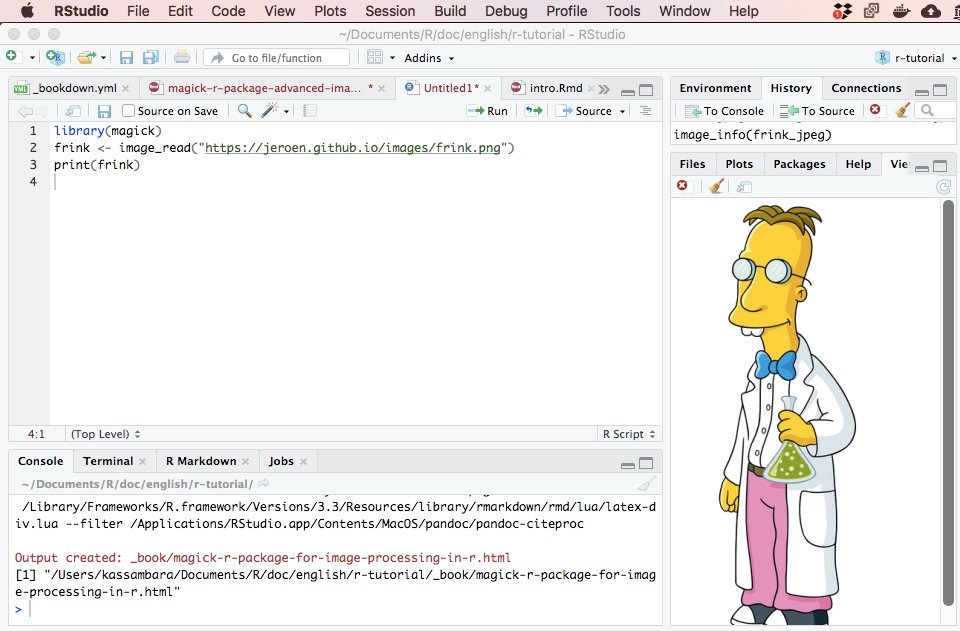
Image transformations
Cut and edit
Several of the transformation functions take an geometry parameter which requires a special syntax of the form AxB+C+D where each element is optional. Some examples:
image_trim(image): Trims margin.image_crop(image, geometry = "100x150+50"): crop outwidth:100pxandheight:150pxstarting+50pxfrom the leftimage_scale(image, geometry = "200"): resize proportionally to width:200pximage_scale(image, grometry = "x200"): resize proportionally to height:200pximage_fill(image, color = "blue", point = "+100+200"): flood fill with blue starting at the point atx:100, y:200image_border(frink, color = "red", geometry = "20x10"): adds a border of 20px left+right and 10px top+bottom
Change image border and background:
# Add 20px left/right and 10px top/bottom
image_border(image_background(frink, "hotpink"), "#000080", "20x10")
Trim margins:
image_trim(frink)Crop the image. Options are here width:100px and height:150px starting +50px from the left
image_crop(frink, "100x150+50")
Resize the image:
# Width: 300px
image_scale(frink, "300")
# Height: 300px
image_scale(frink, "x300")
Rotate or mirror the image
image_rotate(frink, 45)
image_flip(frink)
image_flop(frink)
Modulate and paint an image:
# Change the brightness, the saturation and the Hue
image_modulate(frink, brightness = 80, saturation = 120, hue = 90)

# Paint the shirt in blue
image_fill(frink, "blue", point = "+100+200", fuzz = 20)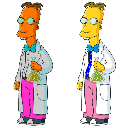
With image_fill we can flood fill starting at pixel point. The fuzz parameter allows for the fill to cross for adjacent pixels with similarish colors. Its value must be between 0 and 256^2 specifying the max geometric distance between colors to be considered equal. Here we give professor frink a blue shirt.
Text annotations
# Add some text
image_annotate(
  frink, text = "I like R!", size = 70, color = "green",
  gravity = "southwest"
  )

# Customize text
image_annotate(
  frink, text = "CONFIDENTIAL", size = 30,
  color = "red", boxcolor = "pink",
  degrees = 60, location = "+50+100",
  font = "Times"
  )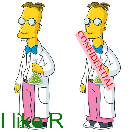
Fonts that are supported on most platforms include "sans", "mono", "serif", "Times", "Helvetica", "Trebuchet", "Georgia", "Palatino"or "Comic Sans".
Layers
Stack layers on top of each other
Import and scale images:
bigdata <- image_read('https://jeroen.github.io/images/bigdata.jpg')
frink <- image_read("https://jeroen.github.io/images/frink.png")
logo <- image_read("https://jeroen.github.io/images/Rlogo.png")
img <- c(bigdata, logo, frink)
img <- image_scale(img, "300x300")
image_info(img)
## format width height colorspace matte filesize
## 1 JPEG 300 225 sRGB FALSE 0
## 2 PNG 300 232 sRGB TRUE 0
## 3 PNG 148 300 sRGB TRUE 0Print images:
# Prints images on top of one another
image_mosaic(img)

# Create a single image which has the size of the first image
image_flatten(img)

# Adding images
image_flatten(img, 'Add')

# Modulate images
image_flatten(img, 'Modulate')

# Minus
image_flatten(img, 'Minus')
Combining or appending images
Put the image frames next to each other:
image_append(image_scale(img, "x200"))
Stack images on top of each other:
image_append(image_scale(img, "100"), stack = TRUE) 
Composing allows for combining two images on a specific position:
bigdatafrink <- image_scale(image_rotate(image_background(frink, "none"), 300), "x200")
image_composite(image_scale(bigdata, "x400"), bigdatafrink, offset = "+180+100")
Create GIF animation
Animating image frames:
image_animate(image_scale(img, "200x200"), fps = 1, dispose = "previous")
Creates a sequence of n images that gradually morph one image into another.
newlogo <- image_scale(image_read("https://jeroen.github.io/images/Rlogo.png"))
oldlogo <- image_scale(image_read("https://developer.r-project.org/Logo/Rlogo-3.png"))
image_resize(c(oldlogo, newlogo), '200x150!') %>%
  image_background('white') %>%
  image_morph() %>%
  image_animate()
Read more
Python Example for Beginners

Two Machine Learning Fields
There are two sides to machine learning:
- Practical Machine Learning:This is about querying databases, cleaning data, writing scripts to transform data and gluing algorithm and libraries together and writing custom code to squeeze reliable answers from data to satisfy difficult and ill defined questions. It’s the mess of reality.
- Theoretical Machine Learning: This is about math and abstraction and idealized scenarios and limits and beauty and informing what is possible. It is a whole lot neater and cleaner and removed from the mess of reality.
Data Science Resources: Data Science Recipes and Applied Machine Learning Recipes
Introduction to Applied Machine Learning & Data Science for Beginners, Business Analysts, Students, Researchers and Freelancers with Python & R Codes @ Western Australian Center for Applied Machine Learning & Data Science (WACAMLDS) !!!
Latest end-to-end Learn by Coding Recipes in Project-Based Learning:
Applied Statistics with R for Beginners and Business Professionals
Data Science and Machine Learning Projects in Python: Tabular Data Analytics
Data Science and Machine Learning Projects in R: Tabular Data Analytics
Python Machine Learning & Data Science Recipes: Learn by Coding
R Machine Learning & Data Science Recipes: Learn by Coding
Comparing Different Machine Learning Algorithms in Python for Classification (FREE)
Disclaimer: The information and code presented within this recipe/tutorial is only for educational and coaching purposes for beginners and developers. Anyone can practice and apply the recipe/tutorial presented here, but the reader is taking full responsibility for his/her actions. The author (content curator) of this recipe (code / program) has made every effort to ensure the accuracy of the information was correct at time of publication. The author (content curator) does not assume and hereby disclaims any liability to any party for any loss, damage, or disruption caused by errors or omissions, whether such errors or omissions result from accident, negligence, or any other cause. The information presented here could also be found in public knowledge domains.