Subplots Python (Matplotlib)

Subplots mean groups of axes that can exist in a single matplotlib figure. subplots() function in the matplotlib library, helps in creating multiple layouts of subplots. It provides control over all the individual plots that are created.

CONTENTS

1. Basic Overview
2. axes() function
3. add_axis() function
4. Creating multiple grids in the same graph
5. Examples using subplot()
6. GridSpec() function
7. tight_layout() function

1. Basic Overview

When analyzing data you might want to compare multiple plots placed side-by-side. Matplotlib provides a convenient method called subplots to do this.

Subplots mean a group of smaller axes (where each axis is a plot) that can exist together within a single figure. Think of a figure as a canvas that holds multiple plots.

Let’s download all the libraries that you will be using.

/* load packages */
import numpy as np
import pandas as pd
import matplotlib.pyplot as plt
%matplotlib inline  

%matplotlib inline ensures that the graphs are displayed in the notebook along with the code.

If you wish to update the default parameters of the matplotlib function, then you need to use plt.rcParams.update() the function available in matplotlib.

/* Set global figure size and dots per inch */
plt.rcParams.update({'figure.figsize':(7,5), 'figure.dpi':100})

There are 3 different ways (at least) to create plots (called axes) in matplotlib. They are:
1. plt.axes()
2. figure.add_axis()
3. plt.subplots()

Of these plt.subplots in the most commonly used. However, the first two approaches are more flexible and allows you to control where exactly on the figure each plot should appear.

To know more plt.subplots(), jump directly to section 4 onwards. However, to understand the whole story, read on.

2. Create a plot inside another plot using axes()

The most basic method of creating axes is to use the plt.axes function.

If you don’t specify any arguments, then you will get only one plot that covers the entire figure.

But if you need to add a subplot, which exists inside another axis, then you can specify the [bottom, left, width,height] to create an axis covering that region.

Calling plt.axes() directly creates a figure object in the background. This is abstracted out for the user.

/* Multiple axis graph */
ax1 = plt.axes() /* standard axes */
ax2 = plt.axes([0.5, 0.5, 0.25, 0.25])

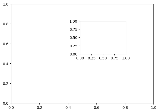
See that there are 2 plots in the same figure. A small plot inside a big plot to be correct.

Let’s plot 2 different functions in the 2 axes.

/* Different functions in different axis */
x= np.arange(0,10,1)
y1 = 5*x -10
y2 = -1*x +3

/* plot */
ax1 = plt.axes() /* standard axes */
ax2 = plt.axes([0.5, 0.5, 0.25, 0.25])
ax1.plot(x,y1)
ax2.plot(x,y2)

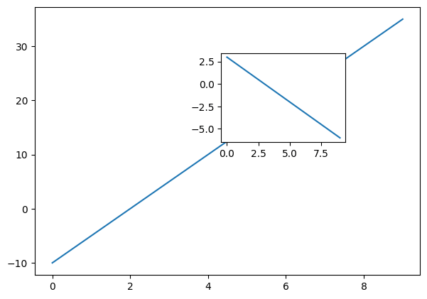
This is the fundamental understanding you need about creating custom axes (or plots).

3. Explicitly create the figure and then do add_axes()

add_axes() is a method of the figure object that is used to add axes (plots) to the figure as per the coordinates you have specified.

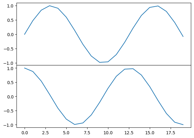
In the below example, let’s draw the sine and cosine graphs in the same figure.

/* create subplots using add_axes */
fig = plt.figure()
ax1 = fig.add_axes([0.1, 0.5, 0.8, 0.4])
ax2 = fig.add_axes([0.1, 0.1, 0.8, 0.4])
x = np.arange(0, 10,0.5)
ax1.plot(np.sin(x))
ax2.plot(np.cos(x))

4. Use plt.subplots to create figure and multiple axes (most useful)

Rather than creating a single axes, this function creates a full grid of equal-sized axes in a single line, returning them in a NumPy array.

You need to specify the no of rows and columns as an argument to the subplots() function.

/* plt.subplots example */
/* Data */
x  = np.arange(0,10,1)
y1 = np.random.randn(10)
y2 = np.random.randn(10)
y3 = np.random.randn(10)
y4 = np.random.randn(10)

/* Create subplots */
fig, ax = plt.subplots(2, 2, sharex='col', sharey='row')
ax[0][0].plot(x,y1)
ax[0][1].plot(x,y2)
ax[1][0].plot(x,y3)
ax[1][1].plot(x,y4)

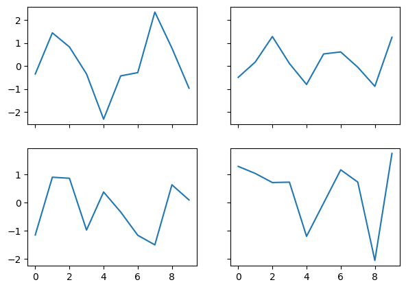
Four plots are drawn in the same graph using random values of y above.

5. Examples using subplots()

Now let’s look into some simple examples on how to draw multiple plots in the same plot.

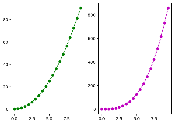
Let’s create an artificial dataset using the np.arange() function. Then, calculate the square and cubic values and plot them in the same graph side-by-side.

I specified the plt.subplots() function arguments to be 1 and 2, so that they are drawn in 1 row but 2 columns.

x =np.arange(0,10,0.5) 
y1 = x*x
y2 = x*x*x
fig, axes = plt.subplots(1, 2) 
axes[0].plot(x, y1, 'g--o') 
axes[1].plot(x, y2, 'm--o')

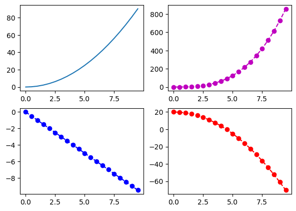
If you want to plot 4 graphs, 2 in each row and 2 in each column, then you need to specify the parameters of plt.subplots() to be 2,2

x =np.arange(0,10,0.5) 
y1 = x*x
y2= x*x*x
y3= -1*x
y4= -x*x +20

fig, axes = plt.subplots(2, 2)  
axes[0, 0].plot(x, y1, '-') 
axes[0, 1].plot(x, y2, 'm--o') 
axes[1, 0].plot(x, y3, 'b--o') 
axes[1, 1].plot(x, y4, 'r--o')

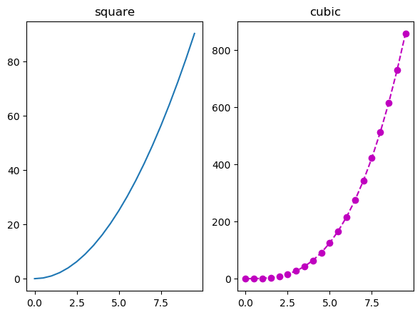
You can also specify the title of each plot using the set_title() method of each axis.

x =np.arange(0,10,0.5) 
y1 = x*x
y2= x*x*x
fig, axes = plt.subplots(1, 2)  
axes[0].plot(x, y1, '-') 
axes[0].set_title('square')
axes[1].plot(x, y2, 'm--o') 
axes[1].set_title('cubic')

6. Using GridSpec() function to create customized axes

plt.GridSpec()is a great command if you want to create grids of different sizes in the same plot.

You need to specify the no. of rows and no. of columns as arguments to the function along with the height and width space.

If you want to create a grid spec for a grid of two rows and two columns with some specified width and height space look like this:

/* Initialize the grid */
grid = plt.GridSpec(2, 3, wspace=0.4, hspace=0.3)

You will see that we can join 2 grids to form one big grid using the,
operator inside the subplot() function.

/* make subplots */
plt.subplot(grid[0, 0])
plt.subplot(grid[0, 1:])
plt.subplot(grid[1, :2])
plt.subplot(grid[1, 2]);

This can be used in a wide variety of cases for plotting multiple plots in matplotlib.

7. Tightly pack the plots with tight_layout()

tight_layout attempts to resize subplots in a figure so that there are no overlaps between axes objects and labels on the axes.

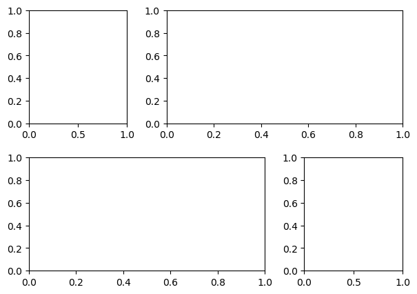
I will create 4 grids in the same plot initially without using the tight_layout function and then including the function to see the difference.

import matplotlib.pyplot as plt
plt.rcParams.update({'figure.figsize':(7.5,5), 'figure.dpi':100})
def plotnew(ax):
    ax.plot([1,2])
    ax.set_xlabel('x-label')
    ax.set_ylabel('y-label')
    ax.set_title('Title')

fig, ((ax1, ax2), (ax3, ax4)) = plt.subplots(nrows=2, ncols=2)
plotnew(ax1)
plotnew(ax2)
plotnew(ax3)
plotnew(ax4)

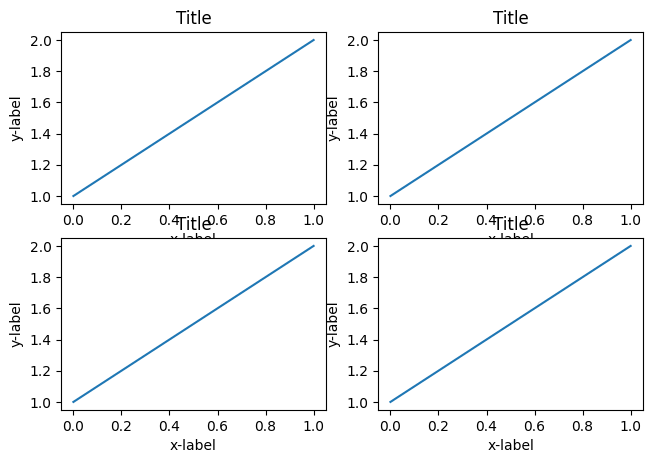
See that in the above plot, there is an overlap between the axis names and the titles of a different plots.

For fixing this, you need to use tight_layout() function.

import matplotlib.pyplot as plt
plt.rcParams.update({'figure.figsize':(7.5,5), 'figure.dpi':100})
def plotnew(ax):
    ax.plot([1,2])
    ax.set_xlabel('x-label')
    ax.set_ylabel('y-label')
    ax.set_title('Title')

fig, ((ax1, ax2), (ax3, ax4)) = plt.subplots(nrows=2, ncols=2)
plotnew(ax1)
plotnew(ax2)
plotnew(ax3)
plotnew(ax4)
plt.tight_layout()

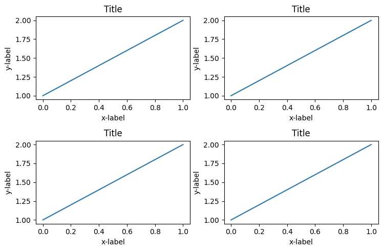
Now you can see that the grids are adjusted perfectly so that there are no overlaps.

Python Example for Beginners

Data Science Resources: Data Science Recipes and Applied Machine Learning Recipes

Introduction to Applied Machine Learning & Data Science for Beginners, Business Analysts, Students, Researchers and Freelancers with Python & R Codes @ Western Australian Center for Applied Machine Learning & Data Science (WACAMLDS) !!!

Latest end-to-end Learn by Coding Recipes in Project-Based Learning:

Applied Statistics with R for Beginners and Business Professionals

Data Science and Machine Learning Projects in Python: Tabular Data Analytics

Data Science and Machine Learning Projects in R: Tabular Data Analytics

Python Machine Learning & Data Science Recipes: Learn by Coding

R Machine Learning & Data Science Recipes: Learn by Coding

Comparing Different Machine Learning Algorithms in Python for Classification (FREE)

Disclaimer: The information and code presented within this recipe/tutorial is only for educational and coaching purposes for beginners and developers. Anyone can practice and apply the recipe/tutorial presented here, but the reader is taking full responsibility for his/her actions. The author (content curator) of this recipe (code / program) has made every effort to ensure the accuracy of the information was correct at time of publication. The author (content curator) does not assume and hereby disclaims any liability to any party for any loss, damage, or disruption caused by errors or omissions, whether such errors or omissions result from accident, negligence, or any other cause. The information presented here could also be found in public knowledge domains.  

Google –> SETScholars