
(Basic Statistics for Citizen Data Scientist)
Measures of Variability
We consider a random variable x and a data set S = {x1, x2, …, xn} of size n which contains possible values of x. The data set can represent either the population being studied or a sample drawn from the population. The mean is the statistic used most often to characterize the center of the data in S. We now consider the following commonly used measures of variability of the data around the mean, namely the standard deviation, variance, squared deviation and average absolute deviation.
In addition we also explore three other measures of variability that are not linked to the mean, namely the median absolute deviation, range and inter-quartile range.
Of these statistics the variance and standard deviation are most commonly employed.
Excel Functions: If R is an Excel range which contains the data elements in S then the Excel function which calculates each of these statistics is shown in Figure 1. Functions marked with an asterisk are supplemental functions found in the Real Statistics Resource Pack, although equivalent formulas in standard Excel are described later.
| Statistic | Excel 2007 | Excel 2010+ | Symbol |
| Population Variance | VARP(R) | VAR.P(R) | σ2 |
| Sample Variance | VAR(R) | VAR.S(R) | s2 |
| Population Standard Deviation | STDEVP(R) | STDEV.P(R) | σ |
| Sample Standard Deviation | STDEV(R) | STDEV.S(R) | s |
| Squared Deviation | DEVSQ(R) | DEVSQ(R) | SS |
| Average Absolute Deviation | AVEDEV(R) | AVEDEV(R) | AAD |
| Median Absolute Deviation | MAD(R) * | MAD(R) * | MAD |
| Range | RNG(R) * | RNG(R) * | |
| Inter-quartile Range | IQR(R, b) * | IQR(R, b) * | IQR |
| Coefficient of Variation | STDEV(R)/AVERAGE(R) | STDEV.S(R)/AVERAGE(R) | V |
Figure 1 – Measures of Variability
Observation: These functions ignore any empty or non-numeric cells.
Variance
Definition 1: The variance is a measure of the dispersion of the data around the mean. Where S represents a population the population variance (symbol σ2) is calculated from the population mean µ as follows:

Where S represents a sample the sample variance (symbol s2) is calculated from the sample mean x̄ as follows:

The reason the expression for the population variance involves division by n while that of the sample variance involves division by n – 1 is explained in Property 3 of Estimators, where division by n – 1 is required to obtained an unbiased estimator of the population variance.
Excel Function: The sample variance is calculated in Excel using the worksheet function VAR. The population variance is calculated in Excel using the function VARP. In Excel 2010/2013 the alternative forms of these functions are VAR.S and VAR.P.
Example 1: If S = {2, 5, -1, 3, 4, 5, 0, 2} represents a population, then the variance = 4.25.
This is calculated as follows. First, the mean = (2+5-1+3+4+5+0+2)/8 = 2.5, and so the squared deviation SS = (2–2.5)2 + (5–2.5)2 + (-1–2.5)2 + (3–2.5)2 + (4–2.5)2 + (5–2.5)2 + (0–2.5)2 + (2–2.5)2 = 34. Thus the variance = SS/n = 34/8 = 4.25
If instead S represents a sample, then the mean is still 2.5, but the variance = SS/(n–1) = 34/7 = 4.86.
These can be calculated in Excel by the formulas VARP(B3;B10) and VAR(B3:B10), as shown in Figure 2.
 Figure 2 – Examples of measures of variability
Observation: When data is expressed in the form of frequency tables then the following properties are useful.
Property 1: If x̄ is the mean of the sample S = {x1, x2, …, xn}, then the sample variance can be expressed by
![]()
Property 2: If µ is the mean of the population S = {x1, x2, …, xn}, then the population variance can be expressed by
![]()
Standard Deviation
Definition 2: The standard deviation is the square root of the variance. Thus the population and sample standard deviations are calculated respectively as follows:

Excel Function: The sample standard deviation is calculated in Excel using the worksheet function STDEV. The population standard deviation is calculated in Excel using the function STDEVP. In Excel 2010/2013 the alternative forms of these functions are STDEV.S and STDEV.P.
Example 2: If S = {2, 5, -1, 3, 4, 5, 0, 2} is a population, then the standard deviation = square root of the population variance = 
If S is a sample, then the sample standard deviation = square root of the sample variance = 
These are the results of the formulas STDEVP(B3:B10) and STDEV(B3:B10), as shown in Figure 2.
Real Statistics Functions: The Real Statistics Resource Pack furnishes the following array functions:
VARCOL(R1) = a row range which contains the sample standard variances of each of the columns in R1
STDEVCOL(R1) = a row range which contains the sample standard deviations of each of the columns in R1
VARROW(R1) = a column range which contains the sample standard variances of each of the rows in R1
STDEVROW(R1) = a column range which contains the sample standard deviations of each of the rows in R1
Example 3: Use the VARCOL and STDEVCOL functions to calculate the sample variance and standard deviation of each of the columns in the range L4:N11 of Figure 3.
The formula =VARCOL(J4:L11) produces the first result (in range J15:L15), while the formula =STDEVCOL(J4:L11) produces the second result (in range J16:L16). Remember that after entering either of these formulas you must press Ctrl-Shft-Enter.
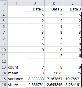
Figure 3 – Sample Variance and Standard Deviation by Column
Property 3: If the population {x1, x2, …, xn} has mean µx and standard deviation σx and the population {y1, y2, …, ym} has mean µy and standard deviation σy, then the variance of the combined population is
![]()
Thus if µx = µy the combined population variance would be
![]()
Property 4: If the sample {x1, x2, …, xn} has mean x̄ and standard deviation sx and the sample {y1, y2, …, ym} has mean ȳ and standard deviation sy, then the variance of the combined sample is
![]()
Thus if x̄ = ȳ, the combined sample variance would be
![]()
Example 4: Find the mean and variance of the sample which results from combining the two samples {3, 4, 6, 7} and {6, 1, 5}.

Figure 4 – Calculation of combined mean and standard deviation
The data in the two samples is given in the range B3:C7 of Figure 4. From these, the mean, variance and standard deviation are calculated for each of the two samples (ranges B12:B15 and C12:C15). Using Property 4, we can calculate the mean and variance of the combined sample (D13 and D14).
If we simply combine the two samples we obtain the data in the range F3:F10, from which we can calculate the mean, variance and standard deviation in the normal way (range D12:D18). As we can see the results are the same.
Observation: In practice instead of using Property 3 and 4, we use the approach shown in the following example, especially since it can be applied to more than two samples or populations.
Example 5: Find the mean and variance of the sample which results from combining the three samples shown in range A3:D6 of Figure 5.

Figure 5 – Calculation of combined mean and variance
We have three samples whose total sample size is 58 (cell B7), calculated via =SUM(B4:B6). The sum of the elements in each sample can be calculated from the mean as shown in range F4:F6. E.g. the sum of all the data elements in sample 1 is 276 (cell F4), calculated via the formula =B4*C4. Thus the sum of all the elements in all three sample is 786 (cell F7), calculated via the formula =SUM(F4:F6). The mean of the combined sample is therefore 13.5517 (cell C7), calculated via the formula =F7/B7.
The calculation of the combined variance is similar. The key is to first find the sum of the squares of all the elements in each sample. These are given in range I4:I6. E.g. the sum of the squares of all the elements in sample 1 is 5512 (cell I4), calculated by =G4+H4 (using Property 1), where G4 contains the formula =B4*C4^2 and H4 contains =(B4-1)*D4. Thus the sum of squares of all the elements in the combined sample is 19,832 (cell I7), calculated by =SUM(I4:I6). Finally, the variance for the combined sample is 161.059 (cell D7), calculated by =(I7-B7*C7^2)/(B7-1), based on Property 1. The standard deviation is therefore 12.6909.
Squared Deviation
Definition 3: The squared deviation (symbol SS for sum of squares) is most often used in ANOVA and related tests. It is calculated as

Excel Function: The squared deviation is calculated in Excel using the worksheet function DEVSQ.
Example 6: If S = {2, 5, -1, 3, 4, 5, 0, 2}, the squared deviation = 34. This is the same as the result of the formula DEVSQ(B3:B10) as shown in Figure 2.
Average Absolute Deviation
Definition 4: The average absolute deviation (AAD) of data set S is calculated as

Excel Function: The average absolute deviation is calculated in Excel using the worksheet function AVEDEV.
Example 7: If S = {2, 5, -1, 3, 4, 5, 0, 2}, the average absolute deviation = 1.75. This is the same as the result of the formula AVEDEV(B3:B10) as shown in Figure 2.
Median Absolute Deviation
Definition 5: The median absolute deviation (MAD) of data set S is calculated as
Median {|xi – 
where
Excel Formula: If R is a range which contains the data elements in S then the MAD of S can be calculated in Excel by the array formula:
=MEDIAN(ABS(R-MEDIAN(R)))
Even though the value is presented in a single cell it is essential that you press Ctrl-Shft-Enter to obtain the array value, otherwise the result won’t come out correctly. This function only works properly when R doesn’t contain any empty cell or cell with a non-numeric value.
Alternatively, you can use the supplemental function MAD(R) which is contained in the Real Statistics Resource Pack. This function works properly even when R contains empty cells and/or cells with non-numeric values. You don’t need to press Ctrl-Shft-Enter to use this function.
Example 8: If S = {2, 5, -1, 3, 4, 5, 0, 2}, the median absolute deviation = 2 since S = {-1, 0, 2, 2, 3, 4, 5, 5}, and so the median of S = (2+3)/2 = 2.5. Thus MAD = the median of {3.5, 2.5, 0.5, 0.5, 0.5, 1.5, 2.5, 2.5} = {0.5, 0.5, 0.5, 1.5, 2.5, 2.5, 2.5, 3.5}, i.e. (1.5+2.5)/2 = 2.
You can achieve the same result using the supplemental formula =MAD(E3:E10) as shown in Figure 2.
Observation: This metric is less affected by extremes in the tails because the data in the tails have less influence on the calculation of the median than they do on the mean.
Range
Definition 6: The range of a data set S is a crude measure of variability and consists simply of the difference between the largest and smallest values in S.
Excel Formula: If R is a range which contains the data elements in S then the range of S can be calculated in Excel by the formula:
=MAX(R) – MIN(R)
Alternatively, you can use the supplemental function RNG(R) which is contained in the Real Statistics Resource Pack.
Example 9: If S = {2, 5, -1, 3, 4, 5, 0, 2}, the range = 5 – (-1) = 6. You can achieve the same result using the supplemental formula =RNG(E3:E10) as shown in Figure 2.
Inter-quartile Range
Definition 7: The inter-quartile range (IQR) of a data set S is calculated as the 75% percentile of S minus the 25% percentile. The IQR provides a rough approximation of the variability near the center of the data in S.
Excel Formula: If R is a range which contains the data elements in S then the IQR of S can be calculated in Excel by the formula:
=QUARTILE(R, 3) – QUARTILE(R, 1)
In Excel 2010/2013 there is a new version of the quartile function called QUARTILE.EXC. An alternative version of IQR is therefore
=QUARTILE.EXC(R, 3) – QUARTILE.EXC(R, 1)
See Ranking Functions in Excel for further information about the QUARTILE and QUARTILE.EXC functions. Alternatively, you can calculate the inter-quartile range via the supplemental function IQR(R, b) which is contained in the Real Statistics Resource Pack. When b = FALSE (default), the first version of IQR is returned, while when b = TRUE the second version is returned.
Example 10: If S = {2, 5, -1, 3, 4, 5, 0, 2}, then the first version of IQR = 4.25 – 1.5 = 2.75, while the second version is IQR = 4.75 – 0.5 = 4.25. You can achieve the same result using the Real Statistics formulas =IQR(B3:B10) and =IQR(B3:B10,TRUE), as shown in Figure 2.
Observation: The variance, standard deviation, average absolute deviation and median absolute deviation measure both the variability near the center and the variability in the tails of the distribution which represents the data. The average absolute deviation and median absolute deviation do not give undue weight to the tails. On the other hand, the range only uses the two most extreme points and the interquartile range only uses the middle portion of the data.
Coefficient of Variation
Definition 8: The coefficient of variation (aka the coefficient of variability), V (or CV), of the data set S is calculated as
V = s/x̄
Since s and x̄ have the same units of measurement, V has no units of measurement. This statistic only makes sense for ratio scale data. The higher the value of V the more dispersion there is.
Clearly, the coefficient of variation is only defined when the mean is not zero.
Excel Formula: If R is a range which contains the data elements in S then the coefficient of variation for S can be calculated in Excel by the formula:
=STDEV.S(R)/AVERAGE(R)
The population version of V is σ/μ which can be calculated in Excel by the formula
=STDEV.P(R)/AVERAGE(R)
Example 11: If S = {2, 5, -1, 3, 4, 5, 0, 2} represents a sample, then, as we can see from Example 1, the coefficient of variation is
V = s/x̄ = 2.203892/2.5 = 88.16%
Example 12: Stock A has an expected return of 12% with a standard deviation of 9% and stock B has an expected return of 8% with a standard deviation of 5%. Use the coefficient of variation to determine which is the better investment.
Since VA = .09/.12 = .75 and VB = .05/.08 = .625, stock B is considered to be the better investment since its relative risk (equal to its coefficient of variation) is lower.
Statistics for Beginners – Measures of Variability
Disclaimer: The information and code presented within this recipe/tutorial is only for educational and coaching purposes for beginners and developers. Anyone can practice and apply the recipe/tutorial presented here, but the reader is taking full responsibility for his/her actions. The author (content curator) of this recipe (code / program) has made every effort to ensure the accuracy of the information was correct at time of publication. The author (content curator) does not assume and hereby disclaims any liability to any party for any loss, damage, or disruption caused by errors or omissions, whether such errors or omissions result from accident, negligence, or any other cause. The information presented here could also be found in public knowledge domains.
Learn by Coding: v-Tutorials on Applied Machine Learning and Data Science for Beginners
Latest end-to-end Learn by Coding Projects (Jupyter Notebooks) in Python and R:
All Notebooks in One Bundle: Data Science Recipes and Examples in Python & R.
End-to-End Python Machine Learning Recipes & Examples.
End-to-End R Machine Learning Recipes & Examples.
Applied Statistics with R for Beginners and Business Professionals
Data Science and Machine Learning Projects in Python: Tabular Data Analytics
Data Science and Machine Learning Projects in R: Tabular Data Analytics
Python Machine Learning & Data Science Recipes: Learn by Coding
R Machine Learning & Data Science Recipes: Learn by Coding
Comparing Different Machine Learning Algorithms in Python for Classification (FREE)
There are 2000+ End-to-End Python & R Notebooks are available to build Professional Portfolio as a Data Scientist and/or Machine Learning Specialist. All Notebooks are only $29.95. We would like to request you to have a look at the website for FREE the end-to-end notebooks, and then decide whether you would like to purchase or not.