The t distribution provides a good way to perform one-sample tests on the mean when the population variance is not known provided the population is normal or the sample is sufficiently large so that the Central Limit Theorem applies.

It turns out that the t distribution provides good results even when the population is not normal and even when the sample is small, provided the sample data is reasonably symmetrically distributed about the sample mean. This can be determined by graphing the data. The following are indications of symmetry:

• The boxplot is relatively symmetrical; i.e. the median is in the center of the box and the whiskers extend equally in each direction
• The histogram looks symmetrical
• The mean is approximately equal to the median
• The coefficient of skewness is relatively small

Example 1: A weight reduction program claims to be effective in treating obesity. To test this claim 12 people were put on the program and the number of pounds of weight gain/loss was recorded for each person after two years, as shown in columns A and B of Figure 1. Can we conclude that the program is effective?

Figure 1 – One sample t-test

A negative value in column B indicates that the subject gained weight. We judge the program to be effective if there is some weight loss at the 95% significance level. Usually we conduct a two-tailed test since there is risk that the program might actual result in weight gain rather than loss, but for this example we will conduct a one-tailed test (perhaps because we have evidence, e.g. from an earlier study, that overall weight gain is unlikely). Thus our null hypothesis is:

H₀: μ ≤ 0; i.e. the program is not effective

From the box plot in Figure 2 we see that the data is quite symmetric and so we use the t-test even though the sample is small.

Figure 2 – Box plot for sample data

Column E of Figure 1 contains all the formulas required to carry out the t test. Since Excel only displays the values of these formulas, we show each of the formulas (in text format) in column G so that you can see how the calculations are performed.

Thus where range R1 is B4:B15, we see that n = COUNT(R1) = 12, x̄ = AVERAGE(R1) = 4.67, s = STDEV(R1) = 11.15 and std err = s ⁄ = 3.22. From this we see that

with df = 11 degrees of freedom.

Since p-value = TDIST(t, df, 1) = TDIST(1.45, 11, 1) = .088 > .05 = α, the null hypothesis is not rejected. This means there is an 8.8% probability of achieving a value for t this high assuming that the null hypothesis is true, and since 8.8% > 5% we can’t reject the null hypothesis.

The same conclusion is reached since

t_crit = TINV(2*α, df) = TINV(.1, 11) = 1.80 > 1.45 = t_obs

Note that if we had used the normal distribution for the hypothesis testing as described in Sampling Distributions we would have gotten the following results:

NORMDIST(x, μ, σ, TRUE) = NORMDIST(4.67, 0, 11.15, TRUE) = .926 < .95 = 1 – α

which would again shows that the null hypothesis can’t be rejected. We see that the probability of being in the critical range is .074 compared to .088 in the t distribution case. In fact, the large sample test (via the normal distribution) is not as accurate as the small sample t distribution test.

Example 2: A school board wanted to see if reading test scores have changed in the past 30 years by testing a random sample of 40 students to see whether there is a significant change from the average score of 78 thirty years ago. The scores of the sample are as follows:

Figure 3 – Random sample data

Based on this data, can we claim that the reading scores have changed in the past 30 years?

From the Histogram data analysis tool we see that the data is reasonably symmetric. This is confirmed by the Descriptive Statistics data analysis tool since the mean and median are approximately equal and the skewness is close to zero (see Figure 4). This justifies the use of a  t test. This time we will perform a two-tailed test.

Figure 4 – Testing for symmetry

We set the null hypothesis to be:

H₀: µ = 78

This time we use the One Sample option of the T Test and Non-parametric Equivalents supplemental data analysis tool provided by the Real Statistics Resource Pack (as described below). The output is shown in Figure 5.

Figure 5 – Real Statistics one sample t test

From the above we see that

with n – 1 = 39 degrees of freedom.

Thus, p-value = TDIST(t, df, 2) = TDIST(3.66, 39, 2) = .00074 < .05 = α, and so we reject the null hypothesis and conclude there is a significant change (i.e. reduction) in test scores.

Alternatively we can calculate, t_crit= TINV(α, df) = TINV(.05, 39) = 2.02. Since |t_obs| = 3.66 > 2.02 =|t_crit|, once again we reject the null hypothesis.

Real Statistics Data Analysis Tool: The Real Statistics Resource Pack provides a supplemental data analysis tool called T Tests and Non-parametric Equivalents, which provides access to the t test for one sample, two independent samples and paired samples, as well as the non-parametric equivalent tests (Mann-Whitney and Wilcoxon Signed-Ranks tests).

For Example 2, enter Ctrl-m and select T Tests and Non-parametric Equivalents from the menu. A dialog box will appear as in Figure 5a.

Figure 5a – Dialog box for T Tests and Non-parametric Equivalents

Enter A5:D14 in the Input Range and 78 for the Hypothetical Mean/Median, unclick Column headings included with data, choose the One sample and T test options and press OK. The output appears in Figure 5. The confidence interval and effect size output in Figure 5 will be described next.

Confidence interval

As described in Confidence Intervals for Sampling Distributions, we can define the confidence interval associated with the t distribution as

Example 3: Calculate the 95% confidence interval for Example 2

This yields a 95% confidence interval of (63.10, 73.70). Since the interval doesn’t contain the hypothetical mean of 78, once again we are justified in rejecting the null hypothesis.

Excel Functions: Versions if Exce starting with Excel 2010 provide the following function to calculate the confidence interval for the t distribution.

CONFIDENCE.T(α, s, n) = k such that (x̄ – k, x̄ + k) is the confidence interval of the sample mean; i.e. CONFIDENCE.T(α, s, n) = t_crit ∙ std error, where n = sample size, s = sample standard deviation and 1 – α is the confidence %.

Thus for Example 2, we calculate CONFIDENCE.T(.05,16.57,40) = 5.30 which yields a 95% confidence interval of (68.40 – 5.30, 68.40 + 5.30) = (63.10, 73.70). The same result was obtained from the T Test and Non-parametric Equivalents data analysis tool, as shown in range D56:T56 of Figure 5.

Observation: Excel’s Descriptive Statistics data analysis tool has an option for generating the confidence interval for a sample or collection of samples using the t distribution. Referring to Figure 2 of Descriptive Statistics Tools, to choose this option click on the Confidence Interval for Mean checkbox and specify the confidence percentage (i.e. 1 – α) if you want to override the default of 95%. E.g. from Figure 4 we see that the 95% confidence interval value in the Descriptive Statistics output for the data in Example 2 is 5.299731.

Real Statistics Excel Functions: The Real Statistics Resource Pack provides the following supplemental functions:

STDERR(R1) = standard error of the data in the range R1 = STDEV(R1) / SQRT(COUNT(R1))

CONFIDENCE_T – equivalent to CONFIDENCE.T (for Excel 2007 and earlier versions)

T_CONF(R1, α) = k such that (x̄ – k, x̄ + k) is the 1 – α confidence interval of the sample mean for the data in range R1 based on the t distribution

T_LOWER(R1, α) = the lower end, x̄ – k, of the 1 – α confidence interval of the sample mean for the data in range R1 based on the t distribution

T_UPPER(R1, α) = the upper end, x̄ + k, of the 1 – α confidence interval of the sample mean for the data in range R1 based on the t distribution

If α is omitted it defaults to .05. These functions ignore any empty or non-numeric cells.

Effect size

As explained in Standardized Effect Size, when the population variance is known we can use Cohen’s d as an estimate of effect size where:

When the population variance is unknown we can use the sample standard deviation as an estimate of the population standard deviation

It turns out that this effect size statistic is biased, especially for small samples (n < 20). An unbiased estimator of the population effect size is given by Hedges’s effect size g.

where df = n – 1 and m = df/2.

Example 4: Calculate the d and g effect sizes for Example 2.

which indicates a medium effect. Except for the sign, this is the same result that was obtained using the T Test and Non-parametric Equivalents data analysis tool (see cell V51 of Figure 5).

Observation: Click here to see how to obtain a confidence interval for Cohen’s effect size.

Observation: In Dichotomous Variables and the t-test, we describe another measure of effect size, namely the correlation coefficient r (which is shown in cell W51 of Figure 5 above), and explain the relationship between r and Cohen’s d.

Statistical Power

We now show how to calculate the power of a t-test using the same approach as we did in Power of a Sample for the normal distribution. In Statistical Power of the t Tests we show another way of computing statistical power using the noncentral t distribution.

Example 5: A university research group wanted to verify the results of a previous study done at another research institution of plants in combating aphids by using a combination of chemicals called Formula Z-protect. The previous study reported that the mean concentration of aphids after an application of Formula Z-protect was 52. The new study examined 20 plants with the concentration of aphids shown on the left side of Figure 6. Determine whether the new study is consistent with the previous results. Also, determine the power of the new study.

We begin by calculating the power for the one-tailed test where the null hypothesis is H₀: μ ≥ 52; later we’ll look at the power of the two-tailed test.

The usual one-sample hypothesis testing is shown on the upper right side of Figure 6a. We now turn our attention to the power analysis, shown on the lower right side of the figure.

Figure 6a – Calculation of power for a one-tailed test

The null hypothesis is rejected provided the sample value is greater than the critical value of t, where t_crit = TINV(α*2, df) = TINV(.05*2, 23) = 1.713872. We double the value of alpha since we are considering the one-tailed test.

Let x_critbe the aphid concentration corresponding to t_crit. Thus,

And so x_crit = 1.713872 ∙ 2.105606 + 52 = 55.60874. We now assume the real population mean is the sample mean, namely 53.16667. As we saw in Power of a Sample, the situation is illustrated in Figure 6, where the curve on the left represents the t distribution being tested with mean μ₀ = 52 and the normal curve on the right represents the distribution with mean μ₁ =53.16667.

Figure 6 – Statistical power

When x_crit = 55.60874, the t statistic for the t distribution with mean 53.16667 is

Thus we have

β = P(t ≤ t_crit | μ = μ₁) = T_DIST(1.159795, 23, TRUE) = 0.870985

And so power = 1 – β = .129015.

Note that T_DIST(t, df, TRUE) is equivalent the following formula:

=IF(t >= 0, TDIST(t, df, 1), 1 – TDIST(-t, df, 1))

or T.DIST(t, df, TRUE) in Excel 2010.

The specific test that was conducted did not reject the null hypothesis, but we also see that such a test would only have found a very small effect of size .1136 (cell G9 of Figure 6a) 12.9% of the time, which is quite poor. Shortly we will consider some of the ways of increasing power to more acceptable levels.

For each value of μ₁ ≥ 52 we can repeat the above calculations to obtain a value of power. From these we obtain the power plot shown in Figure 7.

Figure 7 – Power curve for Example 2

Observation: We are about to conduct a series of what-if analyses. We will use the format shown in Figure 8 for each of these analyses, where the figure repeats the power calculation for Example 2.

Figure 8 – What if analysis (based on given mean)

Example 6: For the data in Example 5, answer the following questions:

1. What is the power of the test for detecting a standardized effect of size .4?
2. What effect size (and mean) can be detected with power .80?
3. What sample size is required to detect an effect of size .2 with power .80?

a) As described above, we use the following measure of effect size:

Thus μ₁ = 752 + (.4)(10.31532) = 56.12612743. As in Example 5, we can then calculate the power of the test to be 59.6% as described in Figure 9:

Figure 9 – Calculating the power of one-tailed t-test

b) We use Excel’s Goal Seek capability to answer the second question. Using the worksheet in Figure 9, we now select Data > Data Tools | What-If Analysis. In the dialog box that appears, enter the following values:

Figure 10 – Dialog box to determine effect size required to obtain power of .80

We are requesting that Excel find the value of cell B10 (the effect size) that produces a value of .8 for cell B13 (the power). Here the first entry must point to a cell that contains a formula. The second entry must be a value and the third entry must point to a cell that contains a value (possibly blank) and not a formula. After clicking on the OK button, a Goal Seek Status dialog box appears, and the worksheet from Figure 9 changes to that in Figure 11.

Figure 11 – Output from Goal Seek to determine effect size

Note that the values of a number of cells have changed to reflect the value necessary to obtain power of .80. In particular, we see that the Effect size (cell B10) contains the value 0.52484634. You must click on the OK button to lock in these new values (or Cancel to return to the original worksheet).

c) We again use Excel’s Goal Seek capability to answer the third question. Using the worksheet in Figure 9 (making sure that the effect size in cell B10 is set to .2), we now enter the following values in the dialog box that appears (see Figure 12):

Figure 12 – Goal Seek dialog box to obtain sample size

After clicking on OK, the worksheet changes to that in Figure 13.

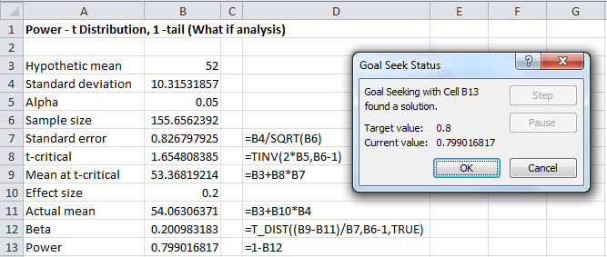
Figure 13 – Output from Goal Seek to determine sample size

In particular, note that the sample size value in cell B6 changes to 155.6562392. Thus the required sample size is 156 (rounding up to the nearest integer).

Example 7: Repeat Example 5 using a two-tailed test, i.e. where the null hypothesis is H₀: μ = 52.

We note that the picture shown in Figure 6 changes to that shown in Figure 14.

Figure 14 – Power for a two-tailed test

The blue curve represents the t distribution assuming that the null hypothesis is true (where μ₀ = 52 for our example). The two critical regions (left and right) are determined by the left and right critical values t_crit. The red curve represents the t distribution assuming that the null hypothesis is false (i.e. the alternative hypothesis is true). For our example we assume that the real population mean is given by the sample mean, i.e. μ₁ = 53.16667. The value of beta is therefore the region bounded by the red curve, the x-axis and the line y = t_-crit and y = t_+crit. Power is then 1−β.

The analysis for Example 7 is shown in Figure 15.

Figure 15 – Calculation of power for a two-tailed t-test

The power for the two-tailed test (cell L15) is 7.9%, which as expected is lower than the power for the one-tailed test.