
(Basic Statistics for Citizen Data Scientist)
Identifying Outliers and Missing Data
The Real Statistics Resource Pack provides an option for identifying potential outliers in a sample. Assuming the sample is normally distributed (based on the Central Limit Theorem), we know that NORM.S.DIST(-2.5,TRUE) = 0.621% of the data should have a z-score less than -2.5. Similarly 0.621% of the data should have a z-score greater than 2.5. Here we use 2.5 as a somewhat arbitrary criteria for a potential outlier. E.g. for a sample of size 80, on average 80(.00621)(2) = .994, or about one element will be viewed as a potential outlier.
Real Statistics Data Analysis Tool: One of the options of the Descriptive Statistics and Normality data analysis tool provided in the Real Statistics Resource Pack is the identification of potential outliers using a specified z-score (default 2.5).
Example 1: Identify potential outliers for the three data samples on the left side of Figure 1 (range B3:D16).

Figure 1 – Identifying potential outliers and missing data
Enter Ctrl-m and select the Descriptive Statistics and Normality data analysis tool. Fill in the dialog box that appears as shown in Figure 2. Leave the Outlier Limit field blank since we want to use the default value of 2.5.
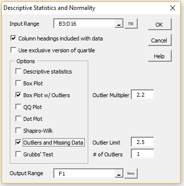
Figure 2 – Dialog box for Descriptive Statistics and Normality
The output as displayed on the right side of Figure 1 shows there are two potential outliers (indicated by the asterisks in column P): namely item 9 of Sample C and item 12 of Sample B. Item 9 of Sample C has a z-score of -2.52391 (cell P17), which is less than -2.5. Item 12 of Sample B has a z-score of 2.62457 (cell N20), which is greater than 2.5.
Note that the z-scores are calculated in the usual way: e.g. the z-score for item 1 of Sample 1 (cell L9) is calculated by the formula =STANDARDIZE(B4, M4, M5).
Note that just because a data element is identified as a potential outlier doesn’t mean that it is wrong or should be eliminated, but it does mean that that data element should be investigated to see if a typing mistake has been made or some other problem has occurred that will distort any analyses that are undertaken.
The output also totals up the number of blank cells (2 for Sample 3) and non-numeric cells (1 for Sample 2, indicated by a series of asterisks in cell N21). These can represent potential missing data.
Observation: Another popularly used method for identifying outliers is to denote any data element larger than Q3 + 1.5*IQR or smaller than Q1 – 1.5*IQR as a potential outlier, where Q1 and Q3 are the first and third quartiles and IQR is the inter-quartile range. This is the approach used in creating box plots.
The box plot displayed in Figure 1 identifies three potential outliers, the two outliers identified above, along with item 4 of Sample A which is just under the 2.5 threshold with a z-score of 2.424183, but does achieve the 1.5*IQR threshold required for the box plot.
Observation: If the Percentage option is set on the Configuration dialog box, then you should enter a value 100 times the desired value in the Outlier Limit field in the dialog box in Figure 2; e.g. enter 300 if you want a 3.0 outlier limit. If you leave this field blank, the outlier limit defaults to 2.5.
Real Statistics Function: The Real Statistics Resource Pack provides the following function, where if type = 0 then the test using the mean and standard deviation is employed while if type = 1 then the test using the IQR is employed.
STANDARD(x, R1, type, exc) takes the value
| STANDARDIZE(x, x̄, s) | if type = 0 (default) | |
| (x−Q3)/IQR | if type = 1 and x > Q3 | |
| (x−Q1)/IQR | if type = 1 and x < Q1 | |
| 0 | otherwise (type = 1 and Q1 ≤ x ≤ Q3) |
where x̄ = AVERAGE(R1) and s = STDEV(R1).
If exc = TRUE then Q1 = QUARTILE.EXC(R1,1) and Q3 = QUARTILE.EXC(R1,3)
If exc = FALSE (default) then Q1 = QUARTILE.INC(R1,1) and Q3 = QUARTILE.INC(R1,3)
The STANDARD function plays a role similar to the STANDARDIZE function when type = 0 (except that the mean and standard deviation are calculated from R1). It plays the equivalent role using the median and IQR when type = 1.
For type = 0, if the value of the STANDARD function at x is larger than 2.5 or less than -2.5 we can consider x to be a potential outlier (although we can change 2.5 to 3.0 or some other value as we choose).
Similarly for type = 1, if the value of the STANDARD function at x is larger than 1.5 or less than -1.5 we can consider x to be a potential outlier (although we can change 1.5 to some other value as we choose).
Example 2: Identify potential outliers for the data set in range B3:D8 of Figure 3.
We insert the formula =STANDARD(B3,$B$3:$D$8) in cell F3, highlight the range F3:H8 and press Ctrl-R and Ctrl-D to fill in the range F3:H8 with the values shown in Figure 3. If we set a cutoff of ±2.5 for outliers, we see that the only value exceeding the cutoff is 2.816972 (cell H5), which means that the data element 99.5 (cell D5) is a potential outlier.
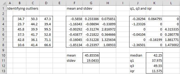
Figure 3 – Identifying potential outliers using the STANDARD function
If we use the type 1 approach instead of the type 0 approach, we insert the formula =STANDARD(B3,$B$3:$D$8,1) in cell J3, highlight the range J3:L8 and press Ctrl-R and Ctrl-D to fill in the range J3:L8 with the values shown in Figure 3. If we set a cutoff of ±1.5 for outliers, we see that the only values exceeding the cutoff are 4.315335 (cell L5) and -2.36501 (cell J8), which means that the data elements 99.5 (cell D5) and 10.6 (cell B8) are potential outliers.
Note that values in the range B3:D8 between Q1 (37.975) and Q3 (49.55) take a zero value in range J3:L8.
Statistics for Beginners in Excel – Identifying Outliers and Missing Data using Real Statistics
Disclaimer: The information and code presented within this recipe/tutorial is only for educational and coaching purposes for beginners and developers. Anyone can practice and apply the recipe/tutorial presented here, but the reader is taking full responsibility for his/her actions. The author (content curator) of this recipe (code / program) has made every effort to ensure the accuracy of the information was correct at time of publication. The author (content curator) does not assume and hereby disclaims any liability to any party for any loss, damage, or disruption caused by errors or omissions, whether such errors or omissions result from accident, negligence, or any other cause. The information presented here could also be found in public knowledge domains.
Learn by Coding: v-Tutorials on Applied Machine Learning and Data Science for Beginners
Latest end-to-end Learn by Coding Projects (Jupyter Notebooks) in Python and R:
All Notebooks in One Bundle: Data Science Recipes and Examples in Python & R.
End-to-End Python Machine Learning Recipes & Examples.
End-to-End R Machine Learning Recipes & Examples.
Applied Statistics with R for Beginners and Business Professionals
Data Science and Machine Learning Projects in Python: Tabular Data Analytics
Data Science and Machine Learning Projects in R: Tabular Data Analytics
Python Machine Learning & Data Science Recipes: Learn by Coding
R Machine Learning & Data Science Recipes: Learn by Coding
Comparing Different Machine Learning Algorithms in Python for Classification (FREE)
There are 2000+ End-to-End Python & R Notebooks are available to build Professional Portfolio as a Data Scientist and/or Machine Learning Specialist. All Notebooks are only $29.95. We would like to request you to have a look at the website for FREE the end-to-end notebooks, and then decide whether you would like to purchase or not.