
(R Tutorials for Business Analyst)
R Data Types, Arithmetic & Logical Operators with Example
- Basic data types
- Variables
- Vectors
- Arithmetic Operators
- Logical Operators
Basic data types
R Programming works with numerous data types, including
- Scalars
- Vectors (numerical, character, logical)
- Matrices
- Data frames
- Lists
Basics types
- 4.5 is a decimal value called numerics.
- 4 is a natural value called integers. Integers are also numerics.
- TRUE or FALSE is a Boolean value called logical.
- The value inside ” ” or ‘ ‘ are text (string). They are called characters.
We can check the type of a variable with the class function.
# Declare variables of different types
# Numeric
x <- 28
class(x)
Output:
## [1] "numeric"
Example 2:
# String
y <- "R is Fantastic"
class(y)
Output:
## [1] "character"
Example 3:
# Boolean
z <- TRUE
class(z)
Output:
## [1] "logical"
Variables
Variables store values and are an important component in programming, especially for a data scientist. A variable can store a number, an object, a statistical result, vector, dataset, a model prediction basically anything R outputs. We can use that variable later simply by calling the name of the variable.
To declare a variable, we need to assign a variable name. The name should not have space. We can use _ to connect to words.
To add a value to the variable, use <- or =.
Here is the syntax:
# First way to declare a variable:  use the `<-`
name_of_variable <- value
# Second way to declare a variable:  use the `=`
name_of_variable = value
In the command line, we can write the following codes to see what happens:
Example 1:
# Print variable x
x <- 42
x
Output:
## [1] 42
Example 2:
y  <- 10
y
Output:
## [1] 10
Example 3:
# We call x and y and apply a subtraction
x-y
Output:
## [1] 32
Vectors
A vector is a one-dimensional array. We can create a vector with all the basic data type we learnt before. The simplest way to build a vector in R, is to use the c command.
Example 1:
# Numerical
vec_num <- c(1, 10, 49)
vec_num
Output:
## [1] 1 10 49
Example 2:
# Character
vec_chr <- c("a", "b", "c")
vec_chr
Output:
## [1] "a" "b" "c"
Example 3:
# Boolean
vec_bool <-  c(TRUE, FALSE, TRUE)
vec_bool
Output:
##[1] TRUE FALSE TRUE
We can do arithmetic calculations on vectors.
Example 4:
# Create the vectors
vect_1 <- c(1, 3, 5)
vect_2 <- c(2, 4, 6)
# Take the sum of A_vector and B_vector
sum_vect <- vect_1 + vect_2
# Print out total_vector
sum_vect
Output:
[1] 3 7 11
Example 5:
In R, it is possible to slice a vector. In some occasion, we are interested in only the first five rows of a vector. We can use the [1:5] command to extract the value 1 to 5.
# Slice the first five rows of the vector
slice_vector <- c(1,2,3,4,5,6,7,8,9,10)
slice_vector[1:5]
Output:
## [1] 1 2 3 4 5
Example 6:
The shortest way to create a range of value is to use the: between two numbers. For instance, from the above example, we can write c(1:10) to create a vector of value from one to ten.
# Faster way to create adjacent values
c(1:10)
Output:
## [1] 1 2 3 4 5 6 7 8 9 10
Arithmetic Operators
We will first see the basic arithmetic operations in R. The following operators stand for:
| Operator | Description |
|---|---|
| + | Addition |
| – | Subtraction |
| * | Multiplication |
| / | Division |
| ^ or ** | Exponentiation |
Example 1:
# An addition
3 + 4
Output:
## [1] 7
You can easily copy and paste the above R code into Rstudio Console. The output is displayed after the character #. For instance, we write the code print(‘Guru99’) the output will be ##[1] Guru99.
The ## means we print an output and the number in the square bracket ([1]) is the number of the display
The sentences starting with # annotation. We can use # inside an R script to add any comment we want. R won’t read it during the running time.
Example 2:
# A multiplication
3*5
Output:
## [1] 15
Example 3:
# A division
(5+5)/2
Output:
## [1] 5
Example 4:
# Exponentiation
2^5
Output:
Example 5:
## [1] 32
# Modulo
28%%6
Output:
## [1] 4
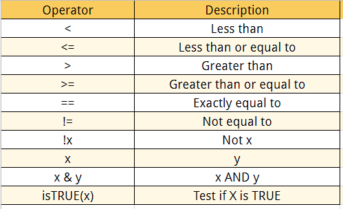
Logical Operators
With logical operators, we want to return values inside the vector based on logical conditions. Following is a detailed list of logical operators available in R
The logical statements in R are wrapped inside the []. We can add many conditional statements as we like but we need to include them in a parenthesis. We can follow this structure to create a conditional statement:
variable_name[(conditional_statement)]
With variable_name referring to the variable, we want to use for the statement. We create the logical statement i.e. variable_name > 0. Finally, we use the square bracket to finalize the logical statement. Below, an example of a logical statement.
Example 1:
# Create a vector from 1 to 10
logical_vector <- c(1:10)
logical_vector>5
Output:
## [1]FALSE FALSE FALSE FALSE FALSE TRUE TRUE TRUE TRUE TRUE
In the output above, R reads each value and compares it to the statement logical_vector>5. If the value is strictly superior to five, then the condition is TRUE, otherwise FALSE. R returns a vector of TRUE and FALSE.
Example 2:
In the example below, we want to extract the values that only meet the condition ‘is strictly superior to five’. For that, we can wrap the condition inside a square bracket precede by the vector containing the values.
# Print value strictly above 5
logical_vector[(logical_vector>5)]
Output:
## [1] 6 7 8 9 10
Example 3:
# Print 5 and 6
logical_vector <- c(1:10)
logical_vector[(logical_vector>4) & (logical_vector<7)]
Output:
## [1] 5 6
Disclaimer: The information and code presented within this recipe/tutorial is only for educational and coaching purposes for beginners and developers. Anyone can practice and apply the recipe/tutorial presented here, but the reader is taking full responsibility for his/her actions. The author (content curator) of this recipe (code / program) has made every effort to ensure the accuracy of the information was correct at time of publication. The author (content curator) does not assume and hereby disclaims any liability to any party for any loss, damage, or disruption caused by errors or omissions, whether such errors or omissions result from accident, negligence, or any other cause. The information presented here could also be found in public knowledge domains.
Learn by Coding: v-Tutorials on Applied Machine Learning and Data Science for Beginners
Latest end-to-end Learn by Coding Projects (Jupyter Notebooks) in Python and R:
All Notebooks in One Bundle: Data Science Recipes and Examples in Python & R.
End-to-End Python Machine Learning Recipes & Examples.
End-to-End R Machine Learning Recipes & Examples.
Applied Statistics with R for Beginners and Business Professionals
Data Science and Machine Learning Projects in Python: Tabular Data Analytics
Data Science and Machine Learning Projects in R: Tabular Data Analytics
Python Machine Learning & Data Science Recipes: Learn by Coding
R Machine Learning & Data Science Recipes: Learn by Coding
Comparing Different Machine Learning Algorithms in Python for Classification (FREE)
There are 2000+ End-to-End Python & R Notebooks are available to build Professional Portfolio as a Data Scientist and/or Machine Learning Specialist. All Notebooks are only $29.95. We would like to request you to have a look at the website for FREE the end-to-end notebooks, and then decide whether you would like to purchase or not.