Python Scatter Plot

Scatter plot is a graph in which the values of two variables are plotted along two axes. It is a most basic type of plot that helps you visualize the relationship between two variables.

Concept

1. What is a Scatter plot?
2. Basic Scatter plot in python
3. Correlation with Scatter plot
4. Changing the color of groups of points
5. Changing the Color and Marker
6. Scatter plot with Linear fit plot using seaborn
7. Scatter Plot with Histograms using seaborn
8. Bubble plot
9. Exploratory Analysis using mtcars Dataset
   • Multiple line of best fits
   • Adjusting color and style for different categories
   • Text Annotation in Scatter Plot
   • Bubble Plot with categorical variables
   • Categorical Plot

What is a Scatter plot?

Scatter plot is a graph of two sets of data along the two axes. It is used to visualize the relationship between the two variables.

If the value along the Y axis seem to increase as X axis increases(or decreases), it could indicate a positive (or negative) linear relationship. Whereas, if the points are randomly distributed with no obvious pattern, it could possibly indicate a lack of dependent relationship.

In python matplotlib, the scatterplot can be created using the pyplot.plot() or the pyplot.scatter(). Using these functions, you can add more feature to your scatter plot, like changing the size, color or shape of the points.

So what is the difference between plt.scatter() vs plt.plot()?

The difference between the two functions is: with pyplot.plot() any property you apply (color, shape, size of points) will be applied across all points whereas in pyplot.scatter() you have more control in each point’s appearance.

That is, in plt.scatter() you can have the color, shape and size of each dot (datapoint) to vary based on another variable. Or even the same variable (y). Whereas, with pyplot.plot(), the properties you set will be applied to all the points in the chart.

First, I am going to import the libraries I will be using.

import pandas as pd
import numpy as np
import matplotlib.pyplot as plt
%matplotlib inline
plt.rcParams.update({'figure.figsize':(10,8), 'figure.dpi':100})

The plt.rcParams.update() function is used to change the default parameters of the plot’s figure.

Basic Scatter plot in python

First, let’s create artifical data using the np.random.randint(). You need to specify the no. of points you require as the arguments.

You can also specify the lower and upper limit of the random variable you need.

Then use the plt.scatter() function to draw a scatter plot using matplotlib. You need to specify the variables x and y as arguments.

plt.title() is used to set title to your plot.

plt.xlabel() is used to label the x axis.

plt.ylabel() is used to label the y axis.

/* Simple Scatterplot */
x = range(50)
y = range(50) + np.random.randint(0,30,50)
plt.scatter(x, y)
plt.rcParams.update({'figure.figsize':(10,8), 'figure.dpi':100})
plt.title('Simple Scatter plot')
plt.xlabel('X - value')
plt.ylabel('Y - value')
plt.show()

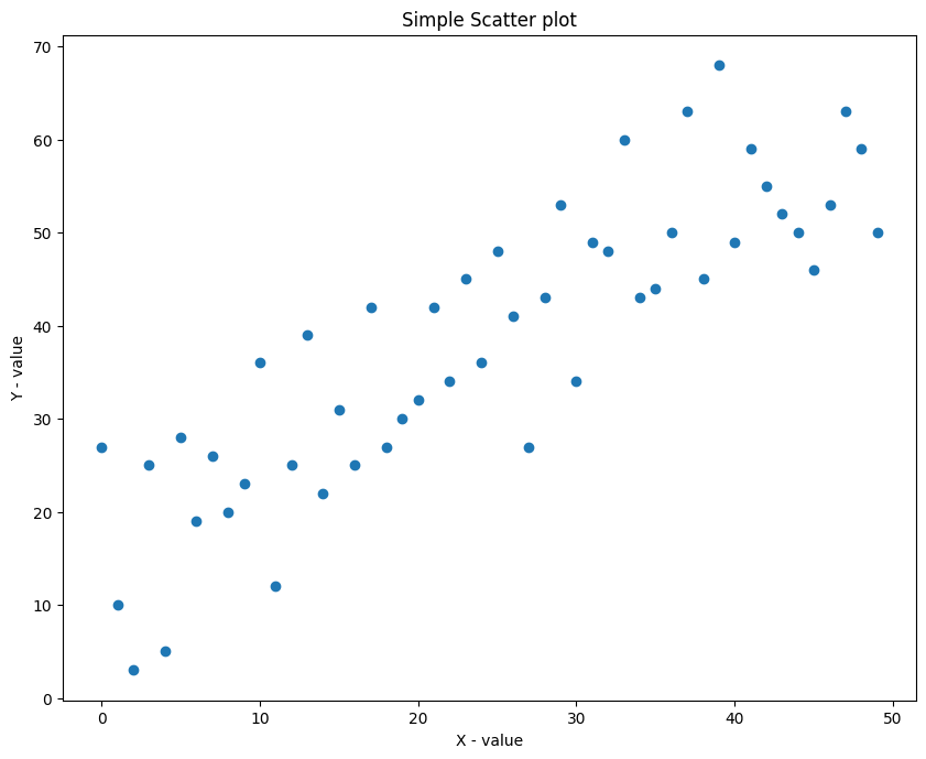
You can see that there is a positive linear relation between the points. That is, as X increases, Y increases as well, because the Y is actually just X + random_number.

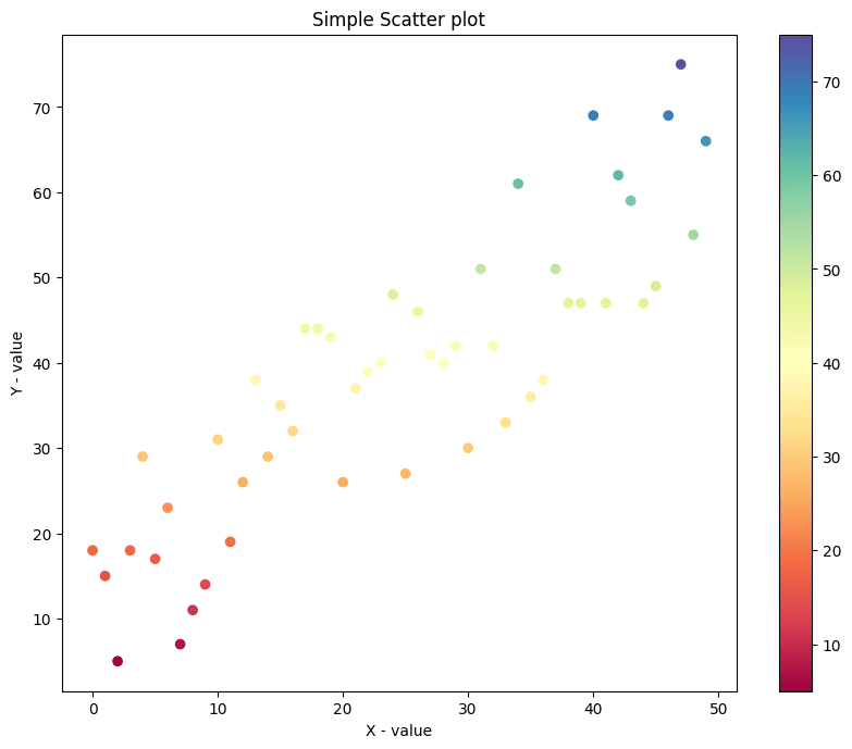
If you want the color of the points to vary depending on the value of Y (or another variable of same size), specify the color each dot should take using the c argument.

You can also provide different variable of same size as X.

/* Simple Scatterplot with colored points */
x = range(50)
y = range(50) + np.random.randint(0,30,50)
plt.rcParams.update({'figure.figsize':(10,8), 'figure.dpi':100})
plt.scatter(x, y, c=y, cmap='Spectral')
plt.colorbar()
plt.title('Simple Scatter plot')
plt.xlabel('X - value')
plt.ylabel('Y - value')
plt.show()

Lets create a dataset with exponentially increasing relation and visualize the plot.

/* Scatterplot of non-random vzriables */
x=np.arange(1,10,0.2)
y= np.exp(x)
plt.scatter(x,y)
plt.rcParams.update({'figure.figsize':(10,8), 'figure.dpi':100})
plt.title('Exponential Relation dataset')
plt.show()

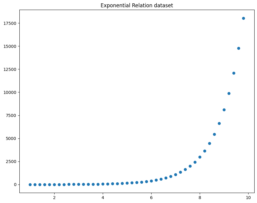
np.arrange(lower_limit, upper_limit, interval) is used to create a dataset between the lower limit and upper limit with a step of ‘interval’ no. of points.

Now you can see that there is a exponential relation between the x and y axis.

Correlation with Scatter plot

1) If the value of y increases with the value of x, then we can say that the variables have a positive correlation.

2) If the value of y decreases with the value of x, then we can say that the variables have a negative correlation.

3) If the value of y changes randomly independent of x, then it is said to have a zero corelation.

/* Scatterplot and Correlations */
/* Data */
x=np.random.randn(100)
y1= x*5 +9 
y2= -5*x
y3=np.random.randn(100)

/* Plot */
plt.rcParams.update({'figure.figsize':(10,8), 'figure.dpi':100})
plt.scatter(x, y1, label=f'y1 Correlation = {np.round(np.corrcoef(x,y1)[0,1], 2)}')
plt.scatter(x, y2, label=f'y2 Correlation = {np.round(np.corrcoef(x,y2)[0,1], 2)}')
plt.scatter(x, y3, label=f'y3 Correlation = {np.round(np.corrcoef(x,y3)[0,1], 2)}')

/* Plot */
plt.title('Scatterplot and Correlations')
plt.legend()
plt.show()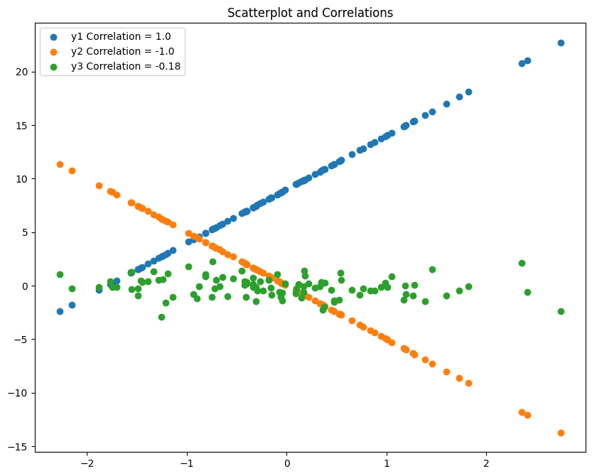

In the above graph, you can see that the blue line shows an positive correlation, the orange line shows a negative corealtion and the green dots show no relation with the x values(it changes randomly independently).

Changing the color of groups of points

Use the color ='____' command to change the colour to represent scatter plot.

/* Scatterplot - Color Change */
x = np.random.randn(50)
y1 = np.random.randn(50)
y2= np.random.randn(50)

/* Plot */
plt.scatter(x,y1,color='blue')
plt.scatter(x,y2,color= 'red')
plt.rcParams.update({'figure.figsize':(10,8), 'figure.dpi':100})

/* Decorate */
plt.title('Color Change')
plt.xlabel('X - value')
plt.ylabel('Y - value')
plt.show()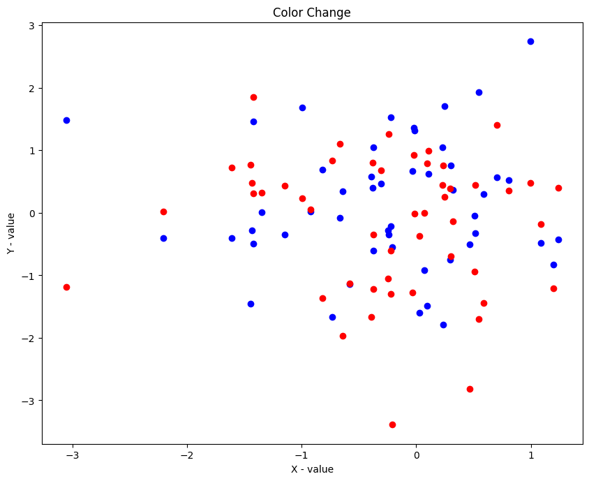

Changing the Color and Marker

Use the marker =_____ command to change the marker type in scatter plot.

[‘.’,’o’,’v’,’^’,’>’,'<‘,’s’,’p’,’*’,’h’,’H’,’D’,’d’,’1′,”,”] – These are the types of markers that you can use for your plot.

/* Scatterplot of different distributions. Color and Shape of Points. */
x = np.random.randn(500)
y1 = np.random.randn(500)
y2 = np.random.chisquare(10, 500)
y3 = np.random.poisson(5, 500)

/* Plot */
plt.rcParams.update({'figure.figsize':(10,8), 'figure.dpi':100})
plt.scatter(x,y1,color='blue', marker= '*', label='Standard Normal')
plt.scatter(x,y2,color= 'red', marker='v', label='Chi-Square')
plt.scatter(x,y3,color= 'green', marker='.', label='Poisson')


/* Decorate */
plt.title('Distributions: Color and Shape change')
plt.xlabel('X - value')
plt.ylabel('Y - value')
plt.legend(loc='best')
plt.show()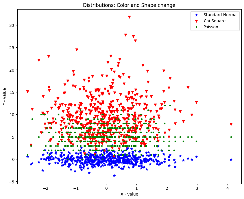

Scatter Plot with Linear fit plot using Seaborn

Lets try to fit the dataset for the best fitting line using the lmplot() function in seaborn.

Lets use the mtcars dataset.

You can download the dataset from the given address: https://www.kaggle.com/ruiromanini/mtcars/download

Now lets try whether there is a linear fit between the mpg and the displ column .

/* Linear - Line of best fit */
import seaborn as sns
url = '/mtcars.csv'
df=pd.read_csv(url)
plt.rcParams.update({'figure.figsize':(10,8), 'figure.dpi':100})
sns.lmplot(x='mpg', y='disp', data=df)
plt.title("Scatter Plot with Linear fit");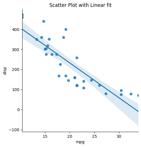

You can see that we are getting a negative corelation between the 2 columns.

/* Scatter Plot with lowess line fit */
url = '/mtcars.csv'
df=pd.read_csv(url)
sns.lmplot(x='mpg', y='disp', data=df, lowess=True) 
plt.title("Scatter Plot with Lowess fit");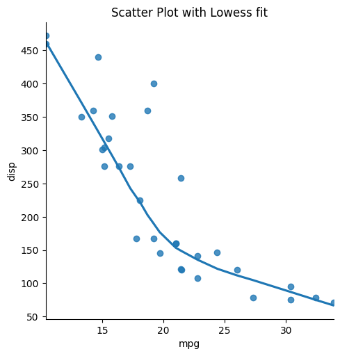

Scatter Plot with Histograms using seaborn

Use the joint plot function in seaborn to represent the scatter plot along with the distribution of both x and y values as historgrams.

Use the sns.jointplot() function with x, y and datset as arguments.

import seaborn as sns
x = np.random.randn(100)
y1 = np.random.randn(100)
plt.rcParams.update({'figure.figsize':(10,8), 'figure.dpi':100})
sns.jointplot(x=x,y=y1);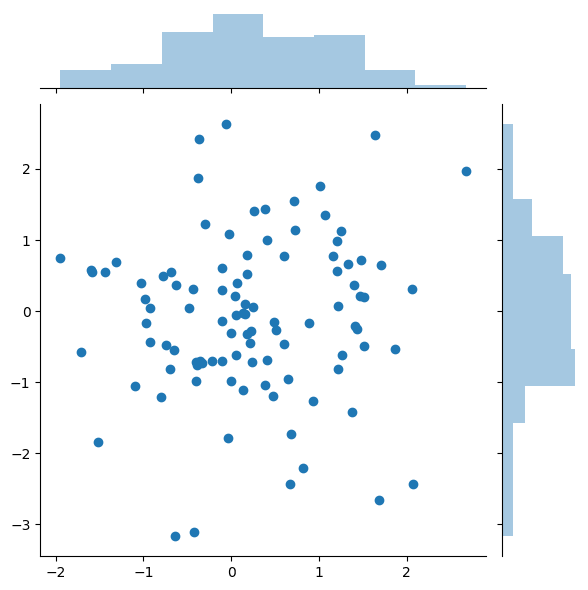

As you can see we are also getting the distribution plot for the x and y value.

Bubble plot

A bubble plot is a scatterplot where a third dimension is added: the value of an additional variable is represented through the size of the dots.

You need to add another command in the scatter plot s which represents the size of the points.

/* Bubble Plot. The size of points changes based on a third varible. */
x = np.random.rand(100)
y = np.random.rand(100)
s = np.random.rand(100)*200
plt.scatter(x, y, s=s,color='red')
plt.show()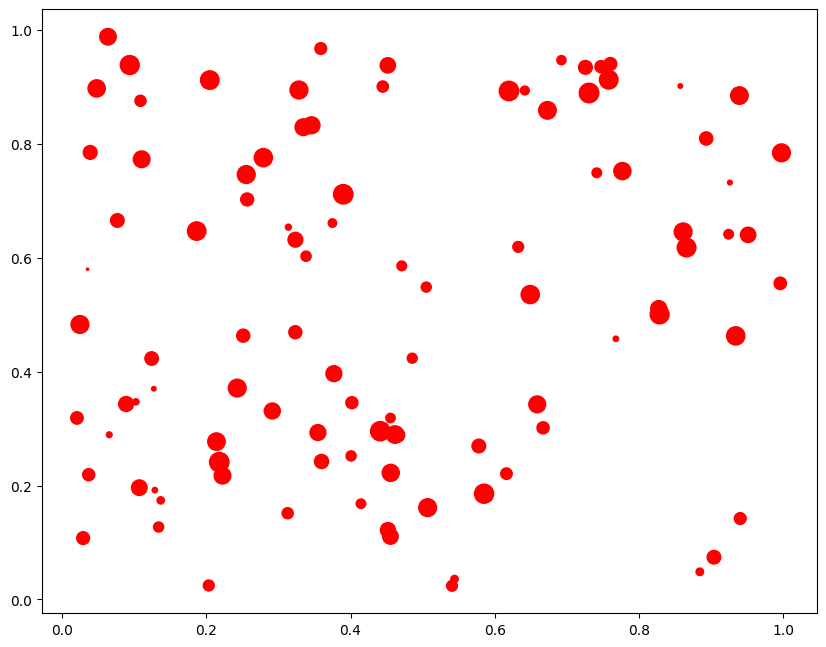

The size of the bubble represents the value of the third dimesnsion, if the bubble size is more then it means that the value of z is large at that point.

Exploratory Analysis of mtcars Dataset

mtcars dataset contains the mileage and vehicle specifications of multiple car models. The dataset can be downloaded here.

The objective of the exploratory analysis is to understand the relationship between the various vehicle specifications and mileage.

df=pd.read_csv("mtcars.csv")
df.head()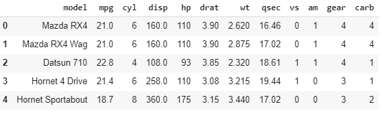

You can see that the dataset contains different informations about a car.

First let’s see a scatter plot to see a distribution between mpg and disp and their histogramic distribution. You can do this by using the jointplot() function in seaborn.

/* joint plot for finding distribution */
sns.jointplot(x=df["mpg"], y=df["disp"],color='red', kind='scatter')

<seaborn.axisgrid.JointGrid at 0x7fbf16fcc5f8>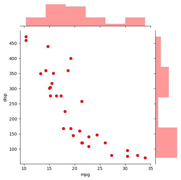

Multiple Line of best fits

If you need to do linear regrssion fit for multiple categories of features between x and y, like in this case, I am further dividing the categories accodring to gear and trying to fit a linear line accordingly. For this, use the hue= argument in the lmplot() function.

/* Linear - Line of best fit */
import seaborn as sns
df=pd.read_csv('mtcars.csv')
plt.rcParams.update({'figure.figsize':(10,8), 'figure.dpi':100})
sns.lmplot(x='mpg', y='disp',hue='gear', data=df);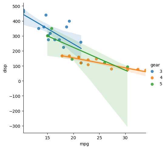

See that the function has fitted 3 different lines for 3 categories of gears in the dataset.

Adjusting color and style for different categories

I splitted the dataset according to different categories of gear. Then I plotted them separately using the scatter() function.

/*  Color and style change according to category */
/* Data */
df=pd.read_csv('mtcars.csv')
df1=df[df['gear']==3]
df2=df[df['gear']==4]
df3=df[df['gear']==5]

/* PLOT */
plt.scatter(df1['mpg'],df1['disp'],color='blue', marker= '*', label='gear=3')
plt.scatter(df2['mpg'],df2['disp'],color= 'red', marker='v', label='gear=4')
plt.scatter(df3['mpg'],df3['disp'],color= 'green', marker='.', label='gear=5')
plt.legend()

<matplotlib.legend.Legend at 0x7fbf171b59b0>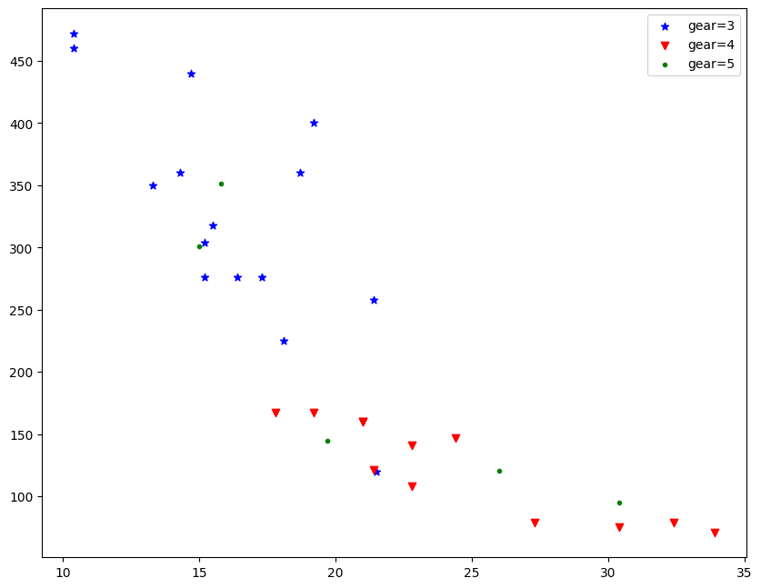

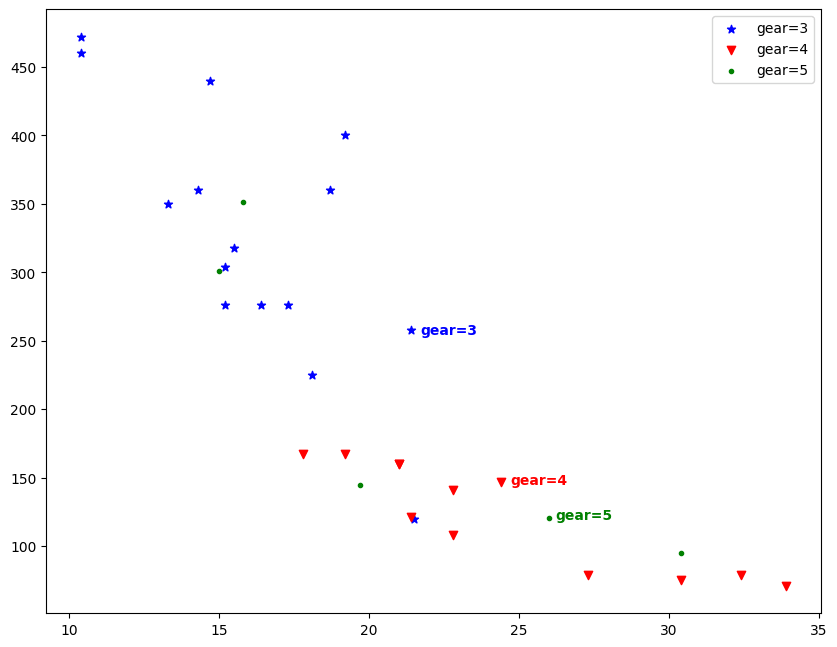
Text Annotation in Scatter Plot

If you need to add any text in your graph use the plt.text() function with the text and the coordinates where you need to add the text as arguments.

/* Text annotation in scatter plot */
df=pd.read_csv('mtcars.csv')
df1=df[df['gear']==3]
df2=df[df['gear']==4]
df3=df[df['gear']==5]

/* Plot */
plt.scatter(df1['mpg'],df1['disp'],color='blue', marker= '*', label='gear=3')
plt.scatter(df2['mpg'],df2['disp'],color= 'red', marker='v', label='gear=4')
plt.scatter(df3['mpg'],df3['disp'],color= 'green', marker='.', label='gear=5')
plt.legend()

/* Text Annotate */
plt.text(21.5+0.2, 255, "gear=3", horizontalalignment='left', size='medium', color='blue', weight='semibold')
plt.text(26+0.2, 120, "gear=5", horizontalalignment='left', size='medium', color='green', weight='semibold')
plt.text(24.5+0.2, 145, "gear=4", horizontalalignment='left', size='medium', color='red', weight='semibold')

Text(24.7, 145, 'gear=4')

Bubble Plot with Categorical Variables

Normally you will use 2 varibales to plot a scatter graph(x and y), then I added another categorical variable df['carb'] which will be implied by the color of the points, I also added another variable df['wt'] whose value will be implied according to the intensity of each color.

/* Bubble Plot */
url = '/mtcars.csv'
df=pd.read_csv(url)

/* Plot */
plt.scatter(df['mpg'],df['disp'],alpha =0.7, s=100* df['wt'], c=df['carb'],cmap='plasma')

/* Decorate */
plt.xlabel('MPG')
plt.ylabel('DISPLACEMENT');
plt.title('Bubble Plot')
plt.legend();

No handles with labels found to put in legend.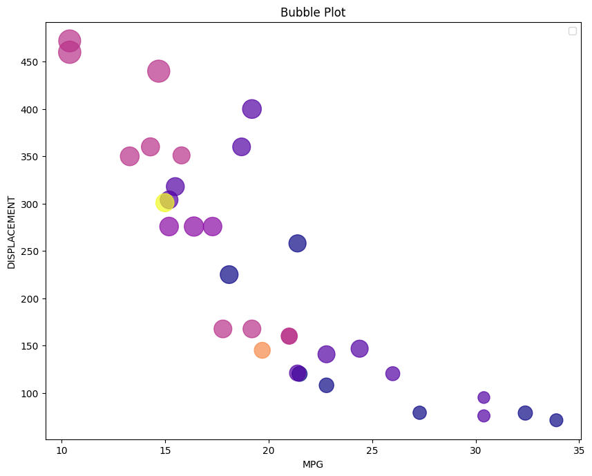

I have plotted the mpg value vs disp value and also splitted them into different colors with respect of carbvalue and the size of each bubble represents the wt value.

alpha paramter is used to chage the color intensity of the plot. More the aplha more will be the color intensity.

Categorical Plot

/* Categorical Plot */
sns.catplot(x="cyl", y="disp", hue="gear", kind="swarm", data=df);
plt.title('Categorical Plot')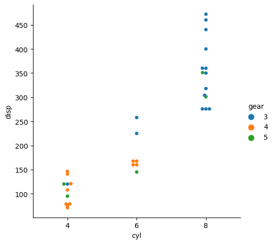

sns.catplot() is used to give access to several axes-level functions that show the relationship between a numerical and one or more categorical variables using one of several visual representations.

Use the hue= command to further split the data into another categories.

Python Example for Beginners

Data Science Resources: Data Science Recipes and Applied Machine Learning Recipes

Introduction to Applied Machine Learning & Data Science for Beginners, Business Analysts, Students, Researchers and Freelancers with Python & R Codes @ Western Australian Center for Applied Machine Learning & Data Science (WACAMLDS) !!!

Latest end-to-end Learn by Coding Recipes in Project-Based Learning:

Applied Statistics with R for Beginners and Business Professionals

Data Science and Machine Learning Projects in Python: Tabular Data Analytics

Data Science and Machine Learning Projects in R: Tabular Data Analytics

Python Machine Learning & Data Science Recipes: Learn by Coding

R Machine Learning & Data Science Recipes: Learn by Coding

Comparing Different Machine Learning Algorithms in Python for Classification (FREE)

Disclaimer: The information and code presented within this recipe/tutorial is only for educational and coaching purposes for beginners and developers. Anyone can practice and apply the recipe/tutorial presented here, but the reader is taking full responsibility for his/her actions. The author (content curator) of this recipe (code / program) has made every effort to ensure the accuracy of the information was correct at time of publication. The author (content curator) does not assume and hereby disclaims any liability to any party for any loss, damage, or disruption caused by errors or omissions, whether such errors or omissions result from accident, negligence, or any other cause. The information presented here could also be found in public knowledge domains.  

Google –> SETScholars