Hash table is a data structure that represents data in the form of key-value pairs. Each key is mapped to a value in the hash table. The keys are used for indexing the values/data. A similar approach is applied by an associative array.

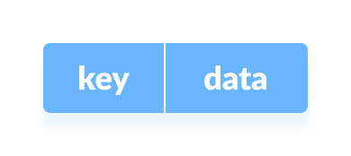
Data is represented in a key value pair with the help of keys as shown in the figure below. Each data is associated with a key. The key is an integer that point to the data.

1. Direct Address Table

Direct address table is used when the amount of space used by the table is not a problem for the program. Here, we assume that

• the keys are small integers
• the number of keys is not too large, and
• no two data have the same key

A pool of integers is taken called universe U = {0, 1, ……., n-1}.

Each slot of a direct address table T[0...n-1] contains a pointer to the element that corresponds to the data.

The index of the array T is the key itself and the content of T is a pointer to the set [key, element]. If there is no element for a key then, it is left as NULL.

Sometimes, the key itself is the data.Pseudocode for operations

directAddressSearch(T, k)
  return T[k]
directAddressInsert(T, x)
  T[x.key] = x
directAddressDelete(T, x)
  T[x.key] = NIL

Limitations of a Direct Address Table

• The value of the key should be small.
• The number of keys must be small enough so that it does not cross the size limit of an array.

2. Hash Table

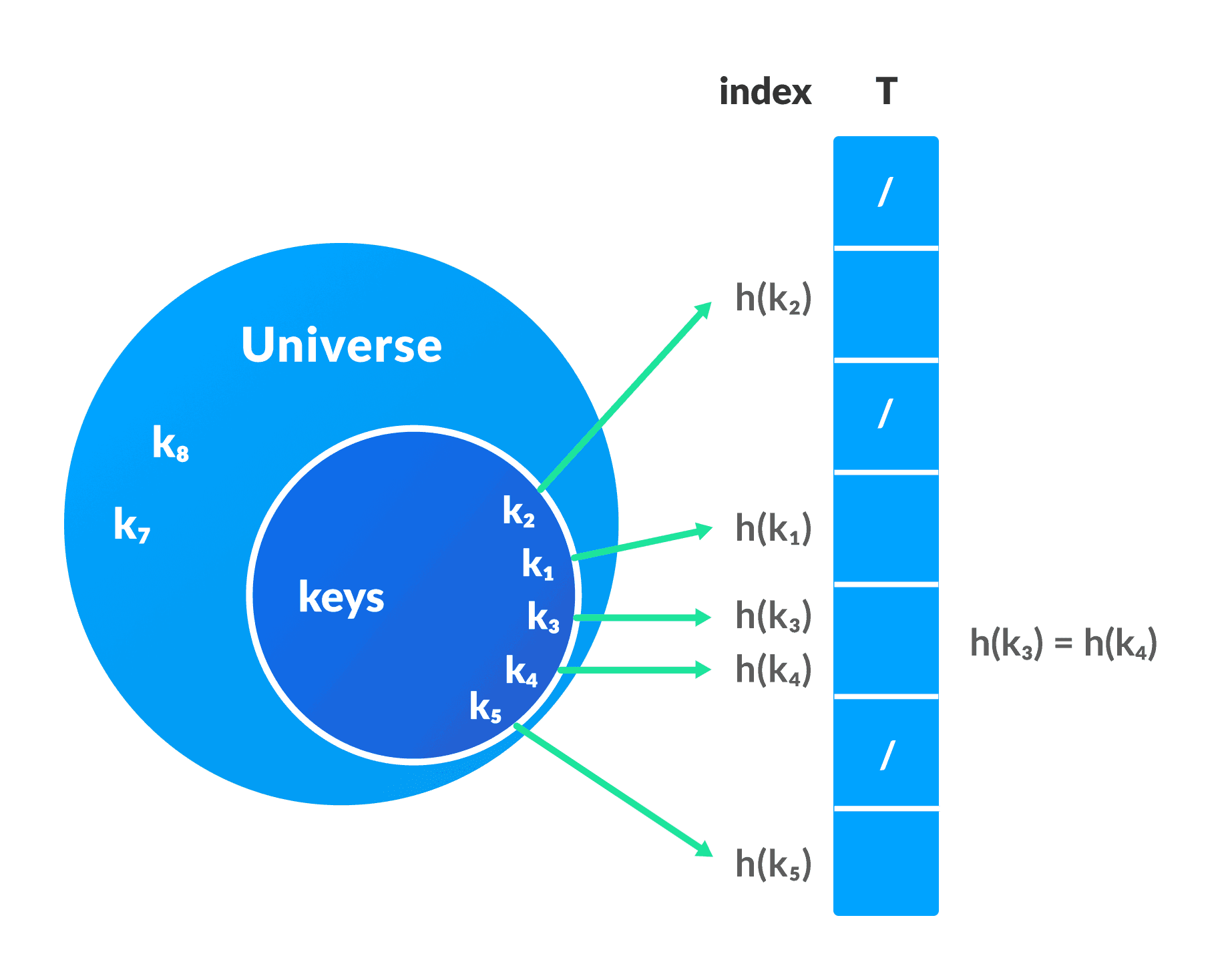
In a hash table, the keys are processed to produce a new index that maps to the required element. This process is called hashing.

Let h(x) be a hash function and k be a key.
h(k) is calculated and it is used as an index for the element.

Limitations of a Hash Table

• If the same index is produced by the hash function for multiple keys then, conflict arises. This situation is called collision.To avoid this, a suitable hash function is chosen. But, it is impossible to produce all unique keys because |U|>m. Thus a good hash function may not prevent the collisions completely however it can reduce the number of collisions.

However, we have other techniques to resolve collision.

Advantages of hash table over direct address table:

The main issues with direct address table are the size of the array and the possibly large value of a key. The hash function reduces the range of index and thus the size of the array is also reduced.
For example, If k = 9845648451321, then h(k) = 11 (by using some hash function). This helps in saving the memory wasted while providing the index of 9845648451321 to the array

Collision resolution by chaining

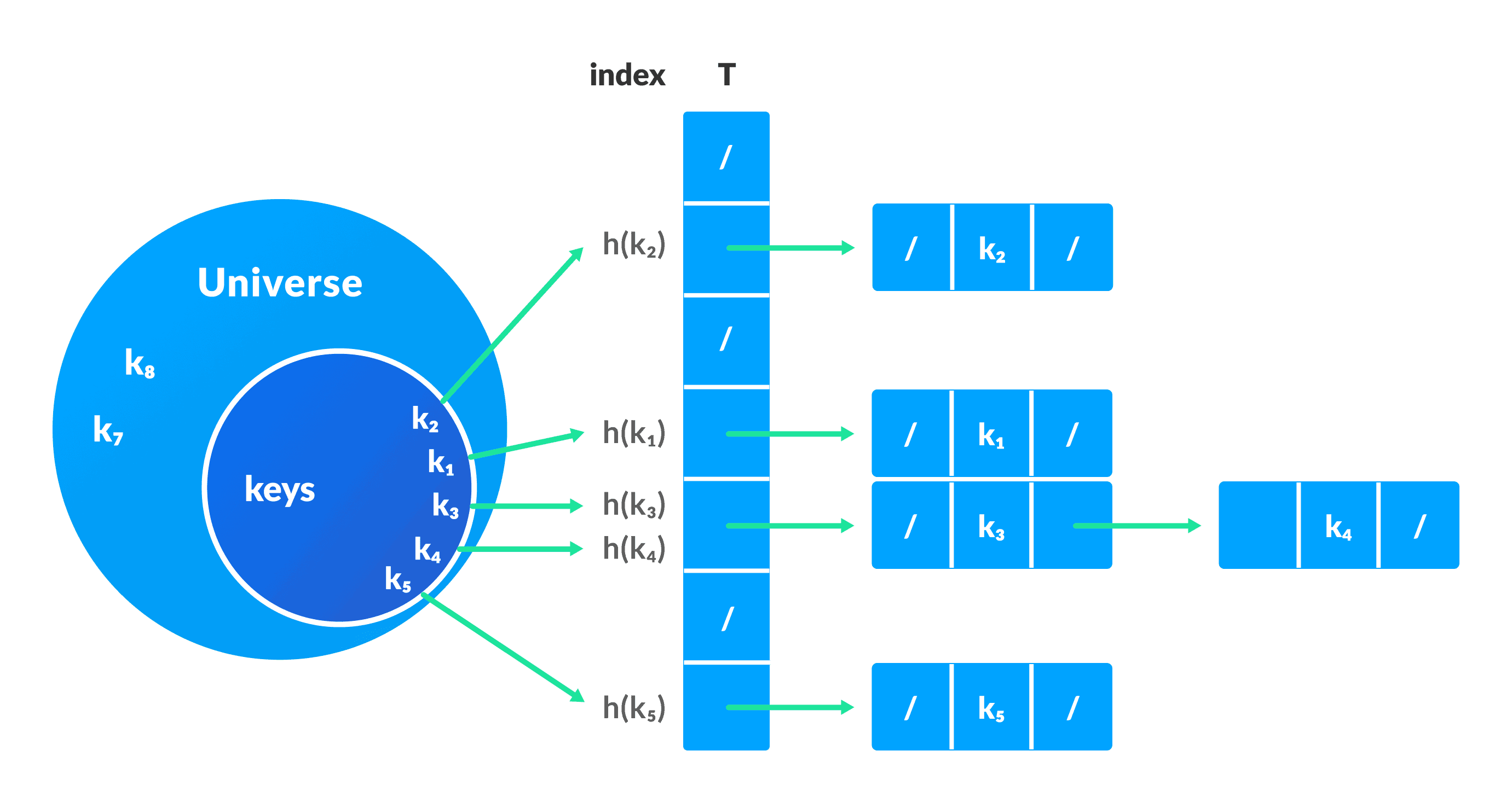
In this technique, if a hash function produces the same index for multiple elements, these elements are stored in the same index by using a doubly linked list.

If j is the slot for multiple elements, it contains a pointer to the head of the list of elements. If no element is present, j contains NIL.

Pseudocode for operations

chainedHashSearch(T, k)
  return T[h(k)]
chainedHashInsert(T, x)
  T[h(x.key)] = x //insert at the head
chainedHashDelete(T, x)
  T[h(x.key)] = NIL

Python Implementation

/* Python program to demonstrate working of HashTable  */

hashTable = [[],] * 10

def checkPrime(n):
    if n == 1 or n == 0:
        return 0

    for i in range(2, n//2):
        if n % i == 0:
            return 0

    return 1


def getPrime(n):
    if n % 2 == 0:
        n = n + 1

    while not checkPrime(n):
        n += 2

    return n


def hashFunction(key):
    capacity = getPrime(10)
    return key % capacity


def insertData(key, data):
    index = hashFunction(key)
    hashTable[index] = [key, data]

def removeData(key):
    index = hashFunction(key)
    hashTable[index] = 0

insertData(123, "apple")
insertData(432, "mango")
insertData(213, "banana")
insertData(654, "guava")

print(hashTable)

removeData(123)

print(hashTable)

Good Hash Functions

A good hash function has the following characteristics.

1. It should not generate keys that are too large and the bucket space is small. Space is wasted.
2. The keys generated should be neither very close nor too far in range.
3. The collision must be minimized as much as possible.

Some of the methods used for hashing are:

Division Method

If k is a key and m is the size of the hash table, the hash function h() is calculated as:

h(k) = k mod m

For example, If the size of a hash table is 10 and k = 112 then h(k) = 112 mod 10 = 2. The value of m must not be the powers of 2. This is because the powers of 2 in binary format are 10, 100, 1000, …. When we find k mod m, we will always get the lower order p-bits.

if m = 22, k = 17, then h(k) = 17 mod 22 = 10001 mod 100 = 01
if m = 23, k = 17, then h(k) = 17 mod 22 = 10001 mod 100 = 001
if m = 24, k = 17, then h(k) = 17 mod 22 = 10001 mod 100 = 0001
if m = 2p, then h(k) = p lower bits of m

Multiplication Method

h(k) = ⌊m(kA mod 1)⌋
where,

• kA mod 1 gives the fractional part kA,
• ⌊ ⌋ gives the floor value
• A is any constant. The value of A lies between 0 and 1. But, an optimal choice will be ≈ (√5-1)/2 suggested by Knuth.

Universal Hashing

In Universal hashing, the hash function is chosen at random independent of keys.

Open Addressing

Multiple values can be stored in a single slot in a normal hash table.

By using open addressing, each slot is either filled with a single key or left NIL. All the elements are stored in the hash table itself.

Unlike chaining, multiple elements cannot be fit into the same slot.

Open addressing is basically a collision resolving technique. Some of the methods used by open addressing are:

Linear Probing

In linear probing, collision is resolved by checking the next slot.
h(k, i) = (h′(k) + i) mod m
where,

• i = {0, 1, ….}
• h'(k) is a new hash function

If a collision occurs at h(k, 0), then h(k, 1) is checked. In this way, the value of i is incremented linearly.
The problem with linear probing is that a cluster of adjacent slots is filled. When inserting a new element, the entire cluster must be traversed. This adds to the time required to perform operations on the hash table.

Quadratic Probing

In quadratic probing, the spacing between the slots is increased (greater than one) by using the following relation.
h(k, i) = (h′(k) + c1i + c2i2) mod m
where,

• c1 and c2 are positive auxiliary constants,
• i = {0, 1, ….}

Double hashing

If a collision occurs after applying a hash function h(k), then another hash function is calculated for finding the next slot.
h(k, i) = (h1(k) + ih2(k)) mod m

Hash Table Applications

Hash tables are implemented where

• constant time lookup and insertion is required
• cryptographic applications
• indexing data is required