Introduction
Time series analysis is a specialized branch of statistics that deals with the analysis of ordered, often temporal data. It is used across a broad range of disciplines, including economics, weather forecasting, finance, and more, to predict future values based on previously observed values. This in-depth guide will take you through the essential concepts and techniques in time series modeling, helping you to understand, analyze, and forecast time series data.
Understanding Time Series Data
Time series data is a sequence of data points indexed in time order. This ordering is typically over equally spaced time intervals, such as minutes, hours, days, months, or years. This sequential nature distinguishes time series data from cross-sectional data, where observations are taken at a single point in time.
Understanding the unique characteristics of time series data is crucial for effective modeling:
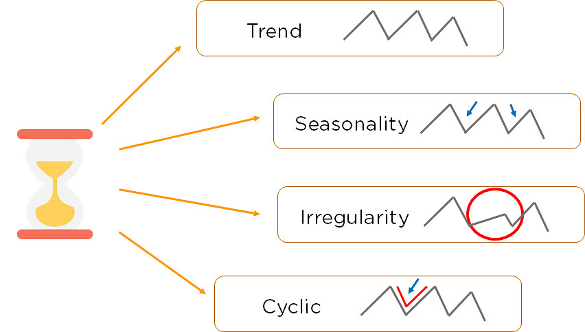
Trend: This is a long-term increase or decrease in the data. A trend can be linear or nonlinear.
Seasonality: This refers to regular, predictable changes in a time series that occur over a specific period, such as daily, monthly, or yearly fluctuations.
Cyclicity: Unlike seasonality, cycles are not of a fixed length. They refer to fluctuations in data that aren’t of a fixed frequency.
Irregularity (or Noise): These are unpredictable, random fluctuations in the data. They are often the residuals or errors in the data after the trend and seasonality are accounted for.
Time Series Decomposition
One of the first steps in time series analysis is to decompose the series into its constituent components: trend, seasonality, and residuals. This can be done using additive or multiplicative models, depending on the nature of the series.
Additive Model: An additive model is used when the components are added together. It is appropriate for time series where the magnitude of the seasonality does not depend on the magnitude of the trend.
Multiplicative Model: A multiplicative model is used when the components are multiplied together. It is appropriate for time series where the magnitude of the seasonality depends on the magnitude of the trend.
Decomposing the time series can provide valuable insights into its underlying patterns and guide the selection of the appropriate forecasting model.
Stationarity in Time Series
Stationarity is a critical concept in time series analysis. A time series is said to be stationary if its statistical properties do not change over time. In other words, it has constant mean, variance, and autocorrelation.
Most time series models require the series to be stationary to make reliable forecasts. If a series is non-stationary, it can often be transformed into a stationary series using techniques such as differencing, logarithmic transformation, or deflation.
Autocorrelation and Partial Autocorrelation
Autocorrelation measures the correlation of a time series with a lagged version of itself. For example, an autocorrelation of order 3 returns the correlation between a time series point and the point three time periods prior. The autocorrelation function (ACF) is a plot of total correlation between different lag functions.
Partial autocorrelation, on the other hand, measures the correlation between a time series and its lags while controlling for the contributions of other lags. The partial autocorrelation function (PACF) can be interpreted as a regression of the series against its past lags.
The ACF and PACF are critical tools for identifying the order of autoregressive (AR), moving average (MA), and AR integrated MA (ARIMA) models.
Time Series Forecasting Models
There are several models used for time series forecasting. The choice of model depends on the nature of the series and the specific business problem at hand. Here are some of the most common time series forecasting models:
Autoregressive (AR) Model: An autoregressive model uses the dependent relationship between an observation and a number of lagged observations. In an AR model, the value of the variable at a time ‘t’ is a linear function of the values at previous time points.
Moving Average (MA) Model: A moving average model uses past forecast errors in a regression-like model. Instead of using past values of the forecast variable in a regression, it uses past forecast errors to predict future values.
Autoregressive Moving Average (ARMA) Model: The ARMA model combines the AR and MA models. It uses the dependent relationship between an observation and a number of lagged observations, as well as the dependency between an observation and a residual error from a moving average model applied to lagged observations.
Autoregressive Integrated Moving Average (ARIMA) Model: The ARIMA model is an extension of the ARMA model that can handle non-stationary data. The ‘integrated’ part of the model (the ‘I’ in ARIMA) refers to the use of differencing to make the time series stationary before the AR and MA parts of the model are applied.
Seasonal Autoregressive Integrated Moving Average (SARIMA) Model: The SARIMA model is an extension of the ARIMA model that supports univariate time series data with a seasonal component. It combines differencing with autoregression and a moving average model to capture the seasonality in the time series data.
Model Selection and Validation
After identifying potential models, the next step is to determine the best model for your data. This involves selecting the model that best captures the characteristics of the time series and provides the most accurate forecasts.
Model selection often involves comparing the performance of different models using a criterion such as the Akaike Information Criterion (AIC) or the Bayesian Information Criterion (BIC). These criteria balance the goodness-of-fit of the model with the complexity of the model.
After a model is selected, it’s important to validate it using a hold-out sample or out-of-sample data. This involves checking the model’s forecast accuracy against actual outcomes. Common measures of forecast accuracy include the Mean Absolute Error (MAE), Mean Squared Error (MSE), and Root Mean Squared Error (RMSE).
Conclusion
Time series analysis is a powerful statistical method for analyzing and forecasting temporal data. With a solid understanding of the key concepts and techniques in time series modeling, including decomposition, stationarity, autocorrelation, and various forecasting models, you can unlock valuable insights from your time series data and make more informed decisions.
Remember that the best model for your data depends on the specific characteristics of your time series and the business context. It’s essential to understand the underlying patterns in your data, choose an appropriate model, and validate the model’s performance to ensure the most accurate forecasts.
With the increasing availability of time-dependent data, time series analysis is becoming an increasingly valuable skill in data science and analytics. By mastering these techniques, you can harness the power of time series data to drive strategic decision-making in your organization.
Find more … …
The Ultimate Guide to Finding Stock Photos and Royalty-Free Images: Top Resources and Tips
Machine Learning for Beginners in Python: How to Use Lag A Time Feature