Introduction: The Significance of Data Exploration in Data Science
Data exploration is a critical first step in any data analysis project, as it allows practitioners to gain insights into the structure, quality, and relationships within a dataset. This process often includes examining summary statistics, visualizing data, identifying outliers and missing values, and performing feature engineering to prepare the data for modeling. In this comprehensive article, we will outline an 11-step guide to data exploration, complete with code examples, to help you effectively analyze and understand your data.
1. Importing Libraries and Loading Data
Begin by importing necessary libraries, such as pandas and numpy, and loading your dataset using pandas’ read_csv() function.
import pandas as pd
import numpy as np

data = pd.read_csv("data.csv")
2. Understanding the Dataset Structure
Examine the structure of the dataset by displaying the first few rows and checking the dimensions, column names, and data types.
data.head()
data.shape
data.columns
data.dtypes
3. Summary Statistics
Calculate summary statistics for the numerical and categorical variables using the describe() and value_counts() functions.
data.describe()
data[“categorical_variable”].value_counts()
4. Identifying Missing Values
Identify missing values in the dataset using the isnull() function, and decide whether to impute or remove these values based on the nature and extent of the missing data.
data.isnull().sum()
5. Univariate Analysis
Perform univariate analysis to examine the distribution of each variable using histograms, box plots, or bar charts.
import matplotlib.pyplot as plt
import seaborn as sns
sns.histplot(data[“numerical_variable”])
sns.boxplot(data[“numerical_variable”])
sns.countplot(data[“categorical_variable”])
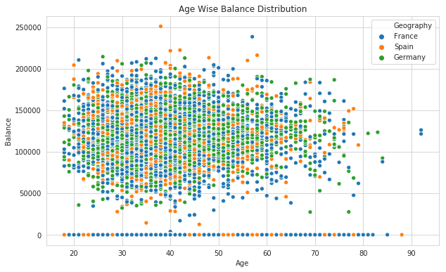
6. Bivariate Analysis
Conduct bivariate analysis to explore the relationships between pairs of variables using scatter plots, correlation matrices, or cross-tabulations.
sns.scatterplot(x=”numerical_variable1", y=”numerical_variable2", data=data)
sns.heatmap(data.corr(), annot=True)
pd.crosstab(data[“categorical_variable1”], data[“categorical_variable2”])
7. Identifying and Treating Outliers
Detect outliers in the dataset using box plots, IQR, or Z-score methods, and decide whether to remove or transform these values based on their impact on the analysis.
Q1 = data[“numerical_variable”].quantile(0.25)
Q3 = data[“numerical_variable”].quantile(0.75)

IQR = Q3 — Q1

outliers = data[(data[“numerical_variable”] < (Q1–1.5 * IQR)) | (data[“numerical_variable”] > (Q3 + 1.5 * IQR))]
8. Feature Engineering
Create new features or transform existing features to improve their relevance or interpretability in the analysis. This may include creating dummy variables, binning, or applying mathematical transformations.
data[“new_feature”] = data[“numerical_variable”] ** 2
data = pd.get_dummies(data, columns=[“categorical_variable”])
9. Feature Scaling
Normalize or standardize numerical features to ensure they are on the same scale, particularly if they will be used as inputs to a machine learning model.
from sklearn.preprocessing import StandardScaler
scaler = StandardScaler()
data[“scaled_numerical_variable”] = scaler.fit_transform(data[[“numerical_variable”]])
10. Dimensionality Reduction
Reduce the dimensionality of the dataset using techniques such as Principal Component Analysis (PCA) or t-distributed Stochastic Neighbor Embedding (t-SNE) to simplify the analysis and improve the performance of machine learning models.
from sklearn.decomposition import PCA
pca = PCA(n_components=2)
data_pca = pca.fit_transform(data[[“numerical_variable1”, “numerical_variable2”]])
11. Saving the Preprocessed Dataset
After completing the data exploration and preprocessing steps, save the cleaned and transformed dataset to a new file for further analysis or modeling.
data.to_csv(“cleaned_data.csv”, index=False)
Conclusion: The Importance of Thorough Data Exploration in Data Science
Data exploration is a vital step in the data science process, as it allows practitioners to understand the quality, structure, and relationships within a dataset. By following this 11-step guide and employing the provided code examples, you can effectively explore and preprocess your data, laying a strong foundation for subsequent analysis and modeling. By mastering data exploration, you can ensure more accurate, reliable, and interpretable results in your data science projects, driving better decision-making and insights across various domains.
Find more … …
Unveiling the Power of Data: A Comprehensive Guide to Data Exploration with R Programming Language