Multiple Linear Regression using Python
Linear Regression:
It is the basic and commonly used type for predictive analysis. It is a statistical approach to modelling the relationship between a dependent variable and a given set of independent variables.
These are of two types:
- Simple linear Regression
- Multiple Linear Regression
Let’s Discuss Multiple Linear Regression using Python.
Multiple Linear Regression attempts to model the relationship between two or more features and a response by fitting a linear equation to observed data. The steps to perform multiple linear Regression are almost similar to that of simple linear Regression. The Difference Lies in the evaluation. We can use it to find out which factor has the highest impact on the predicted output and now different variable relate to each other.
Here : Y = b0 + b1 * x1 + b2 * x2 + b3 * x3 + …… bn * xn
Y = Dependent variable and x1, x2, x3, …… xn = multiple independent variables
Assumption of Regression Model :
- Linearity: The relationship between dependent and independent variables should be linear.
- Homoscedasticity: Constant variance of the errors should be maintained.
- Multivariate normality: Multiple Regression assumes that the residuals are normally distributed.
- Lack of Multicollinearity: It is assumed that there is little or no multicollinearity in the data.
Dummy Variable –
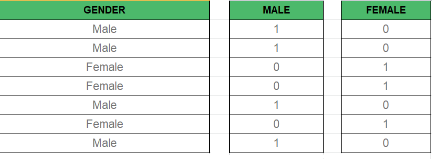
As we know in the Multiple Regression Model we use a lot of categorical data. Using Categorical Data is a good method to include non-numeric data into respective Regression Model. Categorical Data refers to data values which represent categories-data values with the fixed and unordered number of values, for instance, gender(male/female). In the regression model, these values can be represented by Dummy Variables.
These variable consist of values such as 0 or 1 representing the presence and absence of categorical value.

Dummy Variable Trap –
The Dummy Variable Trap is a condition in which two or more are Highly Correlated. In the simple term, we can say that one variable can be predicted from the prediction of the other. The solution of the Dummy Variable Trap is to drop one the categorical variable. So if there are m Dummy variables then m-1 variables are used in the model.
 D2 = D1-1
 Here D2, D1 = Dummy Variables
Method of Building Models :
- All-in
- Backward-Elimination
- Forward Selection
- Bidirectional Elimination
- Score Comparison
Backward-Elimination :
Step #1 : Select a significant level to start in the model.
Step #2 : Fit the full model with all possible predictor.
Step #3 : Consider the predictor with highest P-value. If P > SL go to STEP 4, otherwise model is Ready.
Step #4 : Remove the predictor.
Step #5 : Fit the model without this variable.
Forward-Selection :
Step #1 : Select a significance level to enter the model(e.g. SL = 0.05)
Step #2 : Fit all simple regression models y~ x(n). Select the one with the lowest P-value .
Step #3 : Keep this variable and fit all possible models with one extra predictor added to the one(s) you already have.
Step #4 : Consider the predictor with lowest P-value. If P < SL, go to Step #3, otherwise model is Ready.
Steps Involved in any Multiple Linear Regression Model
Step #1: Data Pre Processing
- Importing The Libraries.
- Importing the Data Set.
- Encoding the Categorical Data.
- Avoiding the Dummy Variable Trap.
- Splitting the Data set into Training Set and Test Set.
Step #2: Fitting Multiple Linear Regression to the Training set
Step #3: Predicting the Test set results.
Code 1 :
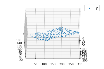
import numpy as np import matplotlib as mpl from mpl_toolkits.mplot3d import Axes3D import matplotlib.pyplot as plt def generate_dataset(n): x = [] y = [] random_x1 = np.random.rand() random_x2 = np.random.rand() for i in range(n): x1 = i x2 = i/2 + np.random.rand()*n x.append([1, x1, x2]) y.append(random_x1 * x1 + random_x2 * x2 + 1) return np.array(x), np.array(y) x, y = generate_dataset(200) mpl.rcParams['legend.fontsize'] = 12 fig = plt.figure() ax = fig.gca(projection ='3d') ax.scatter(x[:, 1], x[:, 2], y, label ='y', s = 5) ax.legend() ax.view_init(45, 0) plt.show() |
Output:

Code 2:
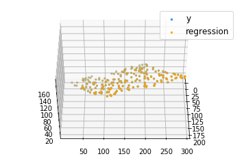
def mse(coef, x, y): return np.mean((np.dot(x, coef) - y)**2)/2 def gradients(coef, x, y): return np.mean(x.transpose()*(np.dot(x, coef) - y), axis = 1) def multilinear_regression(coef, x, y, lr, b1 = 0.9, b2 = 0.999, epsilon = 1e-8): prev_error = 0 m_coef = np.zeros(coef.shape) v_coef = np.zeros(coef.shape) moment_m_coef = np.zeros(coef.shape) moment_v_coef = np.zeros(coef.shape) t = 0 while True: error = mse(coef, x, y) if abs(error - prev_error) <= epsilon: break prev_error = error grad = gradients(coef, x, y) t += 1 m_coef = b1 * m_coef + (1-b1)*grad v_coef = b2 * v_coef + (1-b2)*grad**2 moment_m_coef = m_coef / (1-b1**t) moment_v_coef = v_coef / (1-b2**t) delta = ((lr / moment_v_coef**0.5 + 1e-8) * (b1 * moment_m_coef + (1-b1)*grad/(1-b1**t))) coef = np.subtract(coef, delta) return coef coef = np.array([0, 0, 0]) c = multilinear_regression(coef, x, y, 1e-1) fig = plt.figure() ax = fig.gca(projection ='3d') ax.scatter(x[:, 1], x[:, 2], y, label ='y', s = 5, color ="dodgerblue") ax.scatter(x[:, 1], x[:, 2], c[0] + c[1]*x[:, 1] + c[2]*x[:, 2], label ='regression', s = 5, color ="orange") ax.view_init(45, 0) ax.legend() plt.show() |
Output:

Python Example for Beginners
Two Machine Learning Fields
There are two sides to machine learning:
- Practical Machine Learning:This is about querying databases, cleaning data, writing scripts to transform data and gluing algorithm and libraries together and writing custom code to squeeze reliable answers from data to satisfy difficult and ill defined questions. It’s the mess of reality.
- Theoretical Machine Learning: This is about math and abstraction and idealized scenarios and limits and beauty and informing what is possible. It is a whole lot neater and cleaner and removed from the mess of reality.
Data Science Resources: Data Science Recipes and Applied Machine Learning Recipes
Introduction to Applied Machine Learning & Data Science for Beginners, Business Analysts, Students, Researchers and Freelancers with Python & R Codes @ Western Australian Center for Applied Machine Learning & Data Science (WACAMLDS) !!!
Latest end-to-end Learn by Coding Recipes in Project-Based Learning:
Applied Statistics with R for Beginners and Business Professionals
Data Science and Machine Learning Projects in Python: Tabular Data Analytics
Data Science and Machine Learning Projects in R: Tabular Data Analytics
Python Machine Learning & Data Science Recipes: Learn by Coding
R Machine Learning & Data Science Recipes: Learn by Coding
Comparing Different Machine Learning Algorithms in Python for Classification (FREE)
Disclaimer: The information and code presented within this recipe/tutorial is only for educational and coaching purposes for beginners and developers. Anyone can practice and apply the recipe/tutorial presented here, but the reader is taking full responsibility for his/her actions. The author (content curator) of this recipe (code / program) has made every effort to ensure the accuracy of the information was correct at time of publication. The author (content curator) does not assume and hereby disclaims any liability to any party for any loss, damage, or disruption caused by errors or omissions, whether such errors or omissions result from accident, negligence, or any other cause. The information presented here could also be found in public knowledge domains.
