Linear Regression using sklearn
Linear Regression is a machine learning algorithm based on supervised learning. It performs a regression task. Regression models a target prediction value based on independent variables. It is mostly used for finding out the relationship between variables and forecasting. Different regression models differ based on – the kind of relationship between dependent and independent variables, they are considering and the number of independent variables being used.
This article is going to demonstrate how to use the various Python libraries to implement linear regression on a given dataset. We will demonstrate a binary linear model as this will be easier to visualize.
In this demonstration, the model will use Gradient Descent to learn.
Step 1: Importing all the required libraries
import numpy as np import pandas as pd import seaborn as sns import matplotlib.pyplot as plt from sklearn import preprocessing, svm from sklearn.model_selection import train_test_split from sklearn.linear_model import LinearRegression |
Step 2: Reading the dataset
You can download the dataset here.
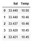
cd C:UsersDevDesktopKaggleSalinity # Changing the file read location to the location of the dataset df = pd.read_csv('bottle.csv') df_binary = df[['Salnty', 'T_degC']] # Taking only the selected two attributes from the dataset df_binary.columns = ['Sal', 'Temp'] # Renaming the columns for easier writing of the code df_binary.head() # Displaying only the 1st rows along with the column names |
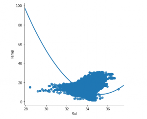
Step 3: Exploring the data scatter
sns.lmplot(x ="Sal", y ="Temp", data = df_binary, order = 2, ci = None) # Plotting the data scatter |
Step 4: Data cleaning
# Eliminating NaN or missing input numbers df_binary.fillna(method ='ffill', inplace = True) |
Step 5: Training our model
X = np.array(df_binary['Sal']).reshape(-1, 1) y = np.array(df_binary['Temp']).reshape(-1, 1) # Separating the data into independent and dependent variables # Converting each dataframe into a numpy array # since each dataframe contains only one column df_binary.dropna(inplace = True) # Dropping any rows with Nan values X_train, X_test, y_train, y_test = train_test_split(X, y, test_size = 0.25) # Splitting the data into training and testing data regr = LinearRegression() regr.fit(X_train, y_train) print(regr.score(X_test, y_test)) |
![]()
Step 6: Exploring our results
y_pred = regr.predict(X_test) plt.scatter(X_test, y_test, color ='b') plt.plot(X_test, y_pred, color ='k') plt.show() # Data scatter of predicted values |
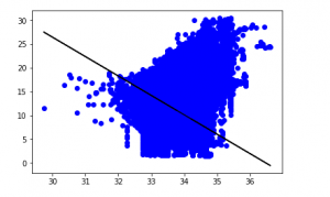
The low accuracy score of our model suggests that our regressive model has not fitted very well to the existing data. This suggests that our data is not suitable for linear regression. But sometimes, a dataset may accept a linear regressor if we consider only a part of it. Let us check for that possibility.
Step 7: Working with a smaller dataset
df_binary500 = df_binary[:][:500] # Selecting the 1st 500 rows of the data sns.lmplot(x ="Sal", y ="Temp", data = df_binary500, order = 2, ci = None) |
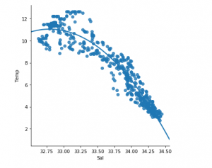
We can already see that the first 500 rows follow a linear model. Continuing with the same steps as before.
df_binary500.fillna(method ='ffill', inplace = True) X = np.array(df_binary500['Sal']).reshape(-1, 1) y = np.array(df_binary500['Temp']).reshape(-1, 1) df_binary500.dropna(inplace = True) X_train, X_test, y_train, y_test = train_test_split(X, y, test_size = 0.25) regr = LinearRegression() regr.fit(X_train, y_train) print(regr.score(X_test, y_test)) |
![]()
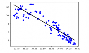
y_pred = regr.predict(X_test) plt.scatter(X_test, y_test, color ='b') plt.plot(X_test, y_pred, color ='k') plt.show() |
Python Example for Beginners
Two Machine Learning Fields
There are two sides to machine learning:
- Practical Machine Learning:This is about querying databases, cleaning data, writing scripts to transform data and gluing algorithm and libraries together and writing custom code to squeeze reliable answers from data to satisfy difficult and ill defined questions. It’s the mess of reality.
- Theoretical Machine Learning: This is about math and abstraction and idealized scenarios and limits and beauty and informing what is possible. It is a whole lot neater and cleaner and removed from the mess of reality.
Data Science Resources: Data Science Recipes and Applied Machine Learning Recipes
Introduction to Applied Machine Learning & Data Science for Beginners, Business Analysts, Students, Researchers and Freelancers with Python & R Codes @ Western Australian Center for Applied Machine Learning & Data Science (WACAMLDS) !!!
Latest end-to-end Learn by Coding Recipes in Project-Based Learning:
Applied Statistics with R for Beginners and Business Professionals
Data Science and Machine Learning Projects in Python: Tabular Data Analytics
Data Science and Machine Learning Projects in R: Tabular Data Analytics
Python Machine Learning & Data Science Recipes: Learn by Coding
R Machine Learning & Data Science Recipes: Learn by Coding
Comparing Different Machine Learning Algorithms in Python for Classification (FREE)
Disclaimer: The information and code presented within this recipe/tutorial is only for educational and coaching purposes for beginners and developers. Anyone can practice and apply the recipe/tutorial presented here, but the reader is taking full responsibility for his/her actions. The author (content curator) of this recipe (code / program) has made every effort to ensure the accuracy of the information was correct at time of publication. The author (content curator) does not assume and hereby disclaims any liability to any party for any loss, damage, or disruption caused by errors or omissions, whether such errors or omissions result from accident, negligence, or any other cause. The information presented here could also be found in public knowledge domains.
