


Introduction: Understanding the Role of Logistic Regression in Data Science
Logistic regression is a widely used statistical method for modeling the relationship between a binary response variable and one or more predictor variables. It is particularly useful for classification tasks, where the goal is to predict which of two categories an observation belongs to. In this extensive article, we will cover the fundamentals of logistic regression, delve into the interpretation of logistic regression coefficients, and explore various applications of this powerful technique in real-world scenarios.
1. Fundamentals of Logistic Regression
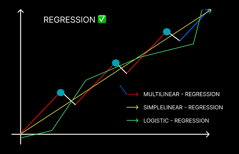
1.1 Logistic Regression vs. Linear Regression
While both logistic and linear regression are used to model the relationship between a response variable and predictor variables, they serve different purposes. Linear regression is used to model continuous response variables, while logistic regression is used to model binary response variables.
1.2 The Logistic Function
The logistic function, also known as the sigmoid function, is the cornerstone of logistic regression. It maps any input value to a value between 0 and 1, representing the probability of an observation belonging to a particular category. The logistic function can be expressed as follows:
P(Y=1) = 1 / (1 + e^(-z))
Where z is a linear combination of the predictor variables, and e is the base of the natural logarithm.
1.3 Maximum Likelihood Estimation
Logistic regression relies on maximum likelihood estimation (MLE) to estimate the coefficients of the predictor variables. MLE is a statistical method that seeks to find the values of the coefficients that maximize the likelihood of observing the data given the model.
2. Interpretation of Logistic Regression Coefficients
2.1 Logit Transformation
To interpret the coefficients of a logistic regression model, it is helpful to use the logit transformation, which is the natural logarithm of the odds ratio. The odds ratio represents the ratio of the probability of an event occurring to the probability of the event not occurring. The logit transformation can be expressed as:
logit(P) = ln(P / (1 — P))
Where P is the probability of an event occurring.
2.2 Interpreting Coefficients
In logistic regression, the coefficients represent the change in the logit of the probability for a one-unit change in the predictor variable, holding all other variables constant. To obtain the odds ratio for a predictor variable, the coefficient can be exponentiated:
Odds Ratio = e^(coefficient)
The odds ratio can then be interpreted as the factor by which the odds of the event occurring change for a one-unit change in the predictor variable.
3. Applications of Logistic Regression
Logistic regression has a wide range of applications across various fields and industries, including:
3.1 Healthcare
In healthcare, logistic regression can be used to predict the likelihood of a patient developing a specific medical condition based on factors such as age, sex, and lifestyle habits. For example, logistic regression can be employed to predict the likelihood of a patient developing diabetes based on their body mass index (BMI), blood pressure, and family history of diabetes.
3.2 Finance
In the financial sector, logistic regression can be utilized to predict the probability of default for credit applicants based on factors such as credit score, employment status, and debt-to-income ratio. This information can help financial institutions make more informed lending decisions and manage risk more effectively.
3.3 Marketing
Logistic regression can be applied in marketing to predict the likelihood of a customer making a purchase or responding to a marketing campaign based on factors such as demographics, past purchase history, and browsing behavior. This information can be used to target marketing efforts more effectively and improve overall campaign performance.
4. Assumptions and Limitations of Logistic Regression
4.1 Assumptions
Logistic regression makes several assumptions, including:
– The response variable is binary: Logistic regression assumes that the response variable has only two possible outcomes (e.g., success/failure or 1/0).
– Independence of observations: The observations in the dataset should be independent of one another.
– Linearity: Logistic regression assumes a linear relationship between the logit of the response variable and the predictor variables.
– Lack of multicollinearity: The predictor variables should not be highly correlated with one another, as this can lead to unstable coefficient estimates and make it difficult to interpret the results.
4.2 Limitations
Despite its many applications, logistic regression has some limitations:
– Restricted to binary outcomes: Logistic regression is not suitable for response variables with more than two categories. However, extensions such as multinomial logistic regression and ordinal logistic regression can be used for these cases.
– Difficulty in capturing complex relationships: If the relationship between the response variable and predictor variables is highly nonlinear or involves complex interactions, logistic regression may not accurately capture these relationships.
– Sensitive to outliers: Logistic regression can be sensitive to outliers in the predictor variables, which can negatively impact the accuracy of the model.
5. Model Evaluation and Improvement
Evaluating the performance of a logistic regression model is crucial to ensure its effectiveness in predicting outcomes. Several metrics and techniques can be used to assess the model’s performance and improve it:
5.1 Confusion Matrix
A confusion matrix is a table that displays the number of true positive, true negative, false positive, and false negative predictions made by the model. This matrix can help calculate various performance metrics, such as accuracy, precision, recall, and F1 score.
5.2 Receiver Operating Characteristic (ROC) Curve
The ROC curve is a graphical representation of the model’s sensitivity (true positive rate) and specificity (true negative rate) across various decision thresholds. The area under the ROC curve (AUC) is a popular performance metric that indicates how well the model can distinguish between the two classes.
5.3 Cross-Validation
Cross-validation is a technique used to assess the generalizability of a model by dividing the dataset into multiple folds and training and testing the model on each fold. This helps to reduce the risk of overfitting and provides a more reliable estimate of the model’s performance.
5.4 Regularization
Regularization is a technique used to prevent overfitting by adding a penalty term to the model’s objective function, which encourages simpler models with smaller coefficients. Lasso (L1) and Ridge (L2) regularization are commonly used in logistic regression to improve model performance and interpretability.
Conclusion: Harnessing the Power of Logistic Regression in Data Science
Logistic regression is a versatile and powerful statistical method for modeling binary response variables and predicting outcomes in a wide range of applications. By understanding the fundamentals of logistic regression, interpreting coefficients, and employing various techniques to evaluate and improve the model’s performance, practitioners can leverage this method to make more informed decisions and drive innovation across various fields and industries.
Find more … …
Hypothesis Testing – Interpreting Data with Statistical Models
Statistics with R for Business Analysts – Logistic Regression