TYPES OF CLUSTERING METHODS: OVERVIEW AND QUICK START R CODE
Clustering methods are used to identify groups of similar objects in a multivariate data sets collected from fields such as marketing, bio-medical and geo-spatial. They are different types of clustering methods, including:
- Partitioning methods
- Hierarchical clustering
- Fuzzy clustering
- Density-based clustering
- Model-based clustering
In this article, we provide an overview of clustering methods and quick start R code to perform cluster analysis in R:
- we start by presenting required R packages and data format for cluster analysis and visualization.
- next, we describe the two standard clustering techniques [partitioning methods (k-MEANS, PAM, CLARA) and hierarchical clustering] as well as how to assess the quality of clustering analysis.
- finally, we describe advanced clustering approaches to find pattern of any shape in large data sets with noise and outliers.
Contents:
- Installing and loading required R packages
- Data preparation
- Distance measures
- Partitioning clustering
- Hierarchical clustering
- Clustering validation and evaluation
- Assessing clustering tendency
- Determining the optimal number of clusters
- Clustering validation statistics
- Advanced clustering methods
- Hybrid clustering methods
- Fuzzy clustering
- Model-based clustering
- DBSCAN: Density-based clustering
Installing and loading required R packages
We’ll use mainly two R packages:
- cluster package: for computing clustering
- factoextra package : for elegant ggplot2-based data visualization.
Accessory packages:
- magrittr for piping: %>%
Install:
install.packages("factoextra")
install.packages("cluster")
install.packages("magrittr")
Load packages:
library("cluster")
library("factoextra")
library("magrittr")
Data preparation
- Demo data set: the built-in R dataset named USArrest
- Remove missing data
- Scale variables to make them comparable
# Load  and prepare the data
data("USArrests")

my_data <- USArrests %>%
  na.omit() %>%          # Remove missing values (NA)
  scale()                # Scale variables

# View the firt 3 rows
head(my_data, n = 3)
## Murder Assault UrbanPop Rape
## Alabama 1.2426 0.783 -0.521 -0.00342
## Alaska 0.5079 1.107 -1.212 2.48420
## Arizona 0.0716 1.479 0.999 1.04288Distance measures
The classification of objects, into clusters, requires some methods for measuring the distance or the (dis)similarity between the objects. Article Clustering Distance Measures Essentials covers the common distance measures used for assessing similarity between observations.
It’s simple to compute and visualize distance matrix using the functions get_dist() and fviz_dist() [factoextra R package]:
get_dist(): for computing a distance matrix between the rows of a data matrix. Compared to the standarddist()function, it supports correlation-based distance measures including “pearson”, “kendall” and “spearman” methods.fviz_dist(): for visualizing a distance matrix
res.dist <- get_dist(USArrests, stand = TRUE, method = "pearson")

fviz_dist(res.dist,
   gradient = list(low = "#00AFBB", mid = "white", high = "#FC4E07"))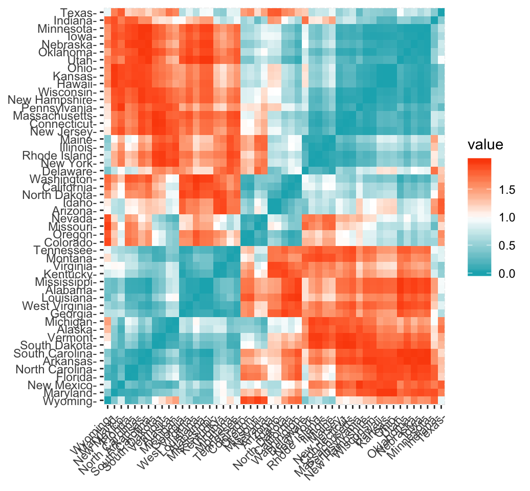
Partitioning clustering
Partitioning algorithms are clustering techniques that subdivide the data sets into a set of k groups, where k is the number of groups pre-specified by the analyst.
There are different types of partitioning clustering methods. The most popular is the K-means clustering (MacQueen 1967), in which, each cluster is represented by the center or means of the data points belonging to the cluster. The K-means method is sensitive to outliers.
An alternative to k-means clustering is the K-medoids clustering or PAM (Partitioning Around Medoids, Kaufman & Rousseeuw, 1990), which is less sensitive to outliers compared to k-means.
Read more: Partitioning Clustering methods.
The following R codes show how to determine the optimal number of clusters and how to compute k-means and PAM clustering in R.
- Determining the optimal number of clusters: use
factoextra::fviz_nbclust()
library("factoextra")
fviz_nbclust(my_data, kmeans, method = "gap_stat")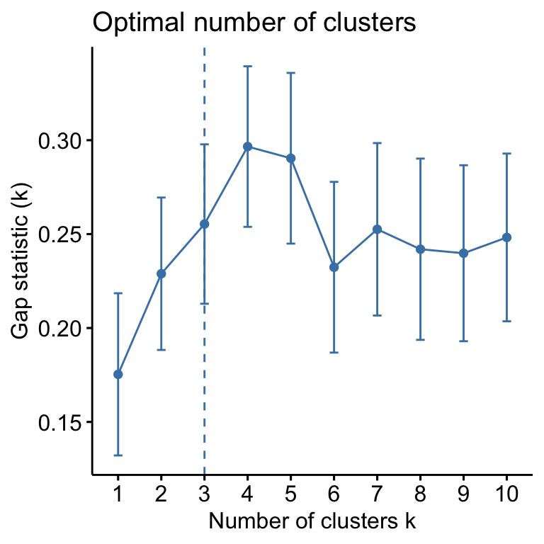
Suggested number of cluster: 3
set.seed(123)
km.res <- kmeans(my_data, 3, nstart = 25)
# Visualize
library("factoextra")
fviz_cluster(km.res, data = my_data,
             ellipse.type = "convex",
             palette = "jco",
             ggtheme = theme_minimal())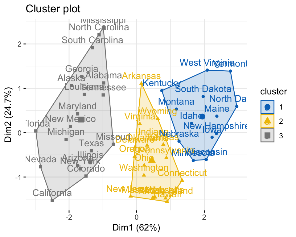
Similarly, the k-medoids/pam clustering can be computed as follow:
# Compute PAM
library("cluster")
pam.res <- pam(my_data, 3)
# Visualize
fviz_cluster(pam.res)
Hierarchical clustering
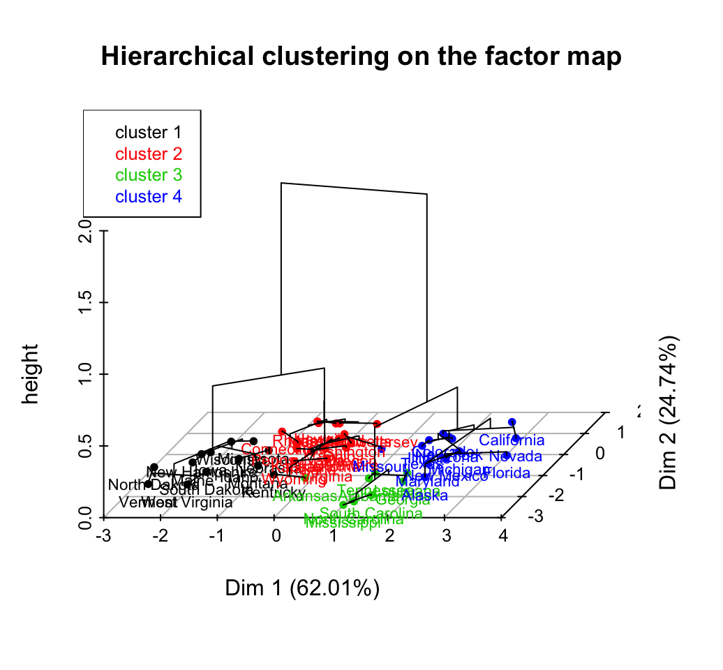
Hierarchical clustering is an alternative approach to partitioning clustering for identifying groups in the dataset. It does not require to pre-specify the number of clusters to be generated.
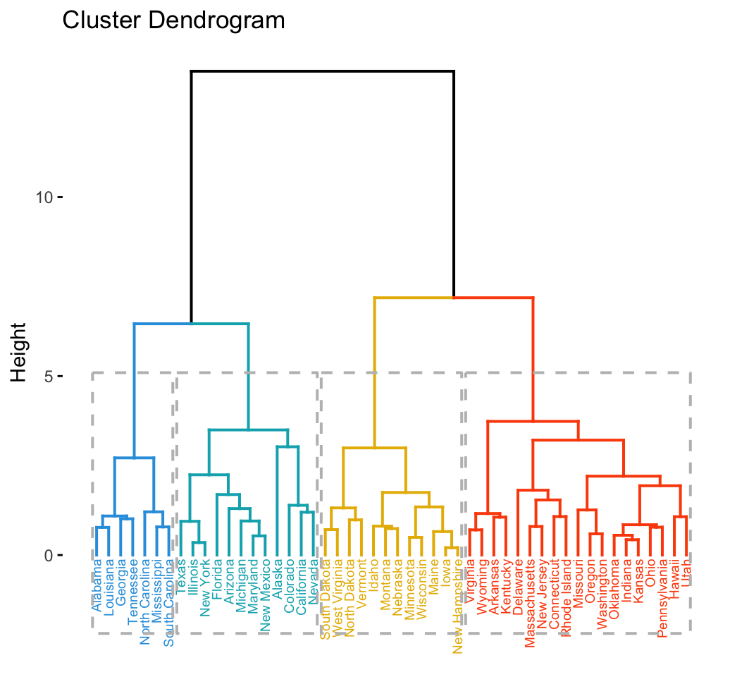
The result of hierarchical clustering is a tree-based representation of the objects, which is also known as dendrogram. Observations can be subdivided into groups by cutting the dendrogram at a desired similarity level.
R code to compute and visualize hierarchical clustering:
# Compute hierarchical clustering
res.hc <- USArrests %>%
  scale() %>%                    # Scale the data
  dist(method = "euclidean") %>% # Compute dissimilarity matrix
  hclust(method = "ward.D2")     # Compute hierachical clustering

# Visualize using factoextra
# Cut in 4 groups and color by groups
fviz_dend(res.hc, k = 4, # Cut in four groups
          cex = 0.5, # label size
          k_colors = c("#2E9FDF", "#00AFBB", "#E7B800", "#FC4E07"),
          color_labels_by_k = TRUE, # color labels by groups
          rect = TRUE # Add rectangle around groups
          )
Clustering validation and evaluation
Clustering validation and evaluation strategies, consist of measuring the goodness of clustering results. Before applying any clustering algorithm to a data set, the first thing to do is to assess the clustering tendency. That is, whether the data contains any inherent grouping structure.
If yes, then how many clusters are there. Next, you can perform hierarchical clustering or partitioning clustering (with a pre-specified number of clusters). Finally, you can use a number of measures, described in this chapter, to evaluate the goodness of the clustering results.
Assessing clustering tendency
To assess the clustering tendency, the Hopkins’ statistic and a visual approach can be used. This can be performed using the function get_clust_tendency() [factoextra package], which creates an ordered dissimilarity image (ODI).
- Hopkins statistic: If the value of Hopkins statistic is close to 1 (far above 0.5), then we can conclude that the dataset is significantly clusterable.
- Visual approach: The visual approach detects the clustering tendency by counting the number of square shaped dark (or colored) blocks along the diagonal in the ordered dissimilarity image.
R code:
gradient.color <- list(low = "steelblue",  high = "white")

iris[, -5] %>%    # Remove column 5 (Species)
  scale() %>%     # Scale variables
  get_clust_tendency(n = 50, gradient = gradient.color)
## $hopkins_stat
## [1] 0.8
##
## $plot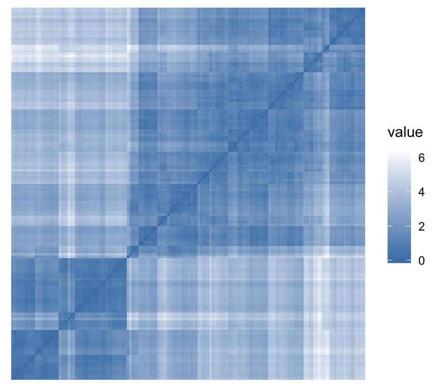
Determining the optimal number of clusters
There are different methods for determining the optimal number of clusters.
In the R code below, we’ll use the NbClust R package, which provides 30 indices for determining the best number of clusters. First, install it using install.packages("NbClust"), then type this:
set.seed(123)

# Compute
library("NbClust")
res.nbclust <- USArrests %>%
  scale() %>%
  NbClust(distance = "euclidean",
          min.nc = 2, max.nc = 10,
          method = "complete", index ="all")
# Visualize
library(factoextra)
fviz_nbclust(res.nbclust, ggtheme = theme_minimal())## Among all indices:
## ===================
## * 2 proposed 0 as the best number of clusters
## * 1 proposed 1 as the best number of clusters
## * 9 proposed 2 as the best number of clusters
## * 4 proposed 3 as the best number of clusters
## * 6 proposed 4 as the best number of clusters
## * 2 proposed 5 as the best number of clusters
## * 1 proposed 8 as the best number of clusters
## * 1 proposed 10 as the best number of clusters
##
## Conclusion
## =========================
## * According to the majority rule, the best number of clusters is 2 .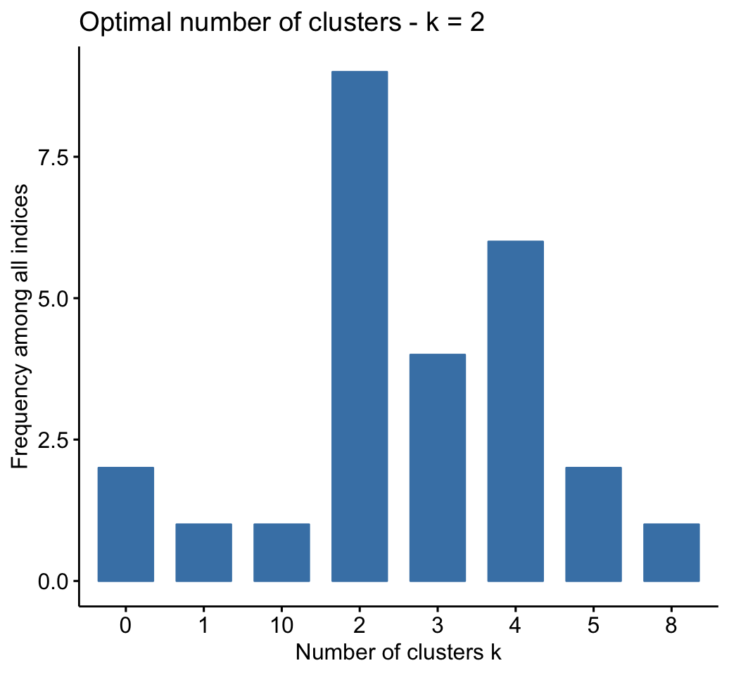
Clustering validation statistics
A variety of measures has been proposed in the literature for evaluating clustering results. The term clustering validation is used to design the procedure of evaluating the results of a clustering algorithm.
The silhouette plot is one of the many measures for inspecting and validating clustering results. Recall that the silhouette (SiSi) measures how similar an object ii is to the the other objects in its own cluster versus those in the neighbor cluster. SiSi values range from 1 to – 1:
- A value of SiSi close to 1 indicates that the object is well clustered. In the other words, the object ii is similar to the other objects in its group.
- A value of SiSi close to -1 indicates that the object is poorly clustered, and that assignment to some other cluster would probably improve the overall results.
In the following R code, we’ll compute and evaluate the result of hierarchical clustering methods.
- Compute and visualize hierarchical clustering:
set.seed(123)
# Enhanced hierarchical clustering, cut in 3 groups
res.hc <- iris[, -5] %>%
  scale() %>%
  eclust("hclust", k = 3, graph = FALSE)

# Visualize with factoextra
fviz_dend(res.hc, palette = "jco",
          rect = TRUE, show_labels = FALSE)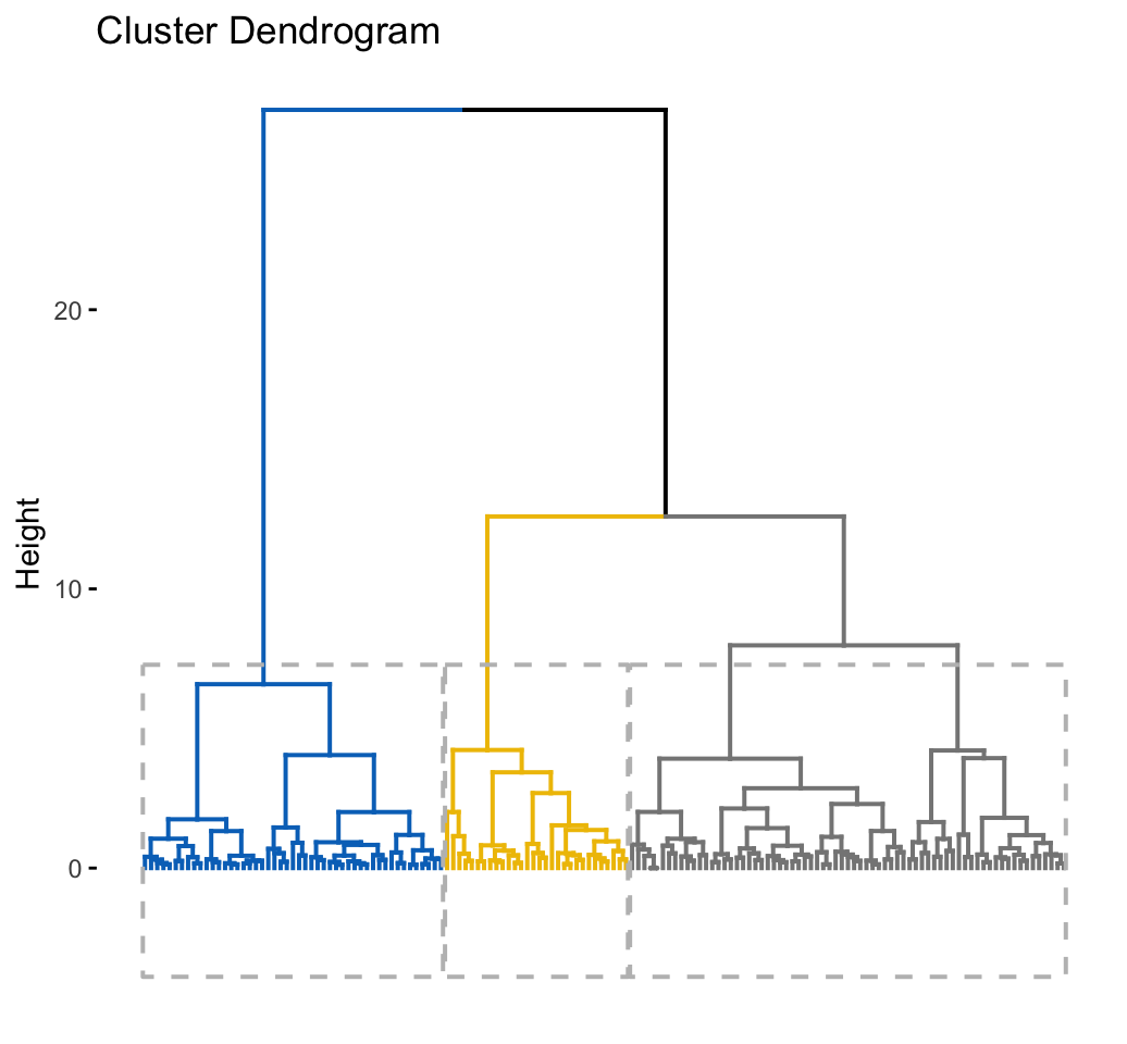
- Inspect the silhouette plot:
fviz_silhouette(res.hc)## cluster size ave.sil.width
## 1 1 49 0.63
## 2 2 30 0.44
## 3 3 71 0.32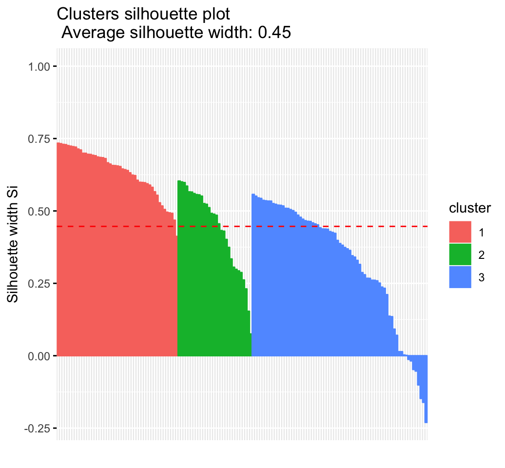
- Which samples have negative silhouette? To what cluster are they closer?
# Silhouette width of observations
sil <- res.hc$silinfo$widths[, 1:3]

# Objects with negative silhouette
neg_sil_index <- which(sil[, 'sil_width'] < 0)
sil[neg_sil_index, , drop = FALSE]
## cluster neighbor sil_width
## 84 3 2 -0.0127
## 122 3 2 -0.0179
## 62 3 2 -0.0476
## 135 3 2 -0.0530
## 73 3 2 -0.1009
## 74 3 2 -0.1476
## 114 3 2 -0.1611
## 72 3 2 -0.2304Advanced clustering methods
Hybrid clustering methods
- Hierarchical K-means Clustering: an hybrid approach for improving k-means results
- HCPC: Hierarchical clustering on principal components
Fuzzy clustering
Fuzzy clustering is also known as soft method. Standard clustering approaches produce partitions (K-means, PAM), in which each observation belongs to only one cluster. This is known as hard clustering.
In Fuzzy clustering, items can be a member of more than one cluster. Each item has a set of membership coefficients corresponding to the degree of being in a given cluster. The Fuzzy c-means method is the most popular fuzzy clustering algorithm.
Model-based clustering
In model-based clustering, the data are viewed as coming from a distribution that is mixture of two ore more clusters. It finds best fit of models to data and estimates the number of clusters.
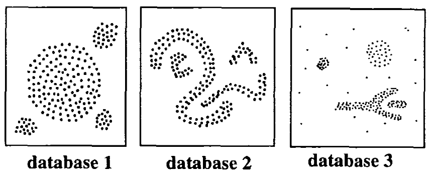
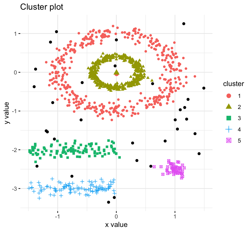
DBSCAN: Density-based clustering
DBSCAN is a partitioning method that has been introduced in Ester et al. (1996). It can find out clusters of different shapes and sizes from data containing noise and outliers (Ester et al. 1996). The basic idea behind density-based clustering approach is derived from a human intuitive clustering method.
Python Example for Beginners

Two Machine Learning Fields
There are two sides to machine learning:
- Practical Machine Learning:This is about querying databases, cleaning data, writing scripts to transform data and gluing algorithm and libraries together and writing custom code to squeeze reliable answers from data to satisfy difficult and ill defined questions. It’s the mess of reality.
- Theoretical Machine Learning: This is about math and abstraction and idealized scenarios and limits and beauty and informing what is possible. It is a whole lot neater and cleaner and removed from the mess of reality.
Data Science Resources: Data Science Recipes and Applied Machine Learning Recipes
Introduction to Applied Machine Learning & Data Science for Beginners, Business Analysts, Students, Researchers and Freelancers with Python & R Codes @ Western Australian Center for Applied Machine Learning & Data Science (WACAMLDS) !!!
Latest end-to-end Learn by Coding Recipes in Project-Based Learning:
Applied Statistics with R for Beginners and Business Professionals
Data Science and Machine Learning Projects in Python: Tabular Data Analytics
Data Science and Machine Learning Projects in R: Tabular Data Analytics
Python Machine Learning & Data Science Recipes: Learn by Coding
R Machine Learning & Data Science Recipes: Learn by Coding
Comparing Different Machine Learning Algorithms in Python for Classification (FREE)
Disclaimer: The information and code presented within this recipe/tutorial is only for educational and coaching purposes for beginners and developers. Anyone can practice and apply the recipe/tutorial presented here, but the reader is taking full responsibility for his/her actions. The author (content curator) of this recipe (code / program) has made every effort to ensure the accuracy of the information was correct at time of publication. The author (content curator) does not assume and hereby disclaims any liability to any party for any loss, damage, or disruption caused by errors or omissions, whether such errors or omissions result from accident, negligence, or any other cause. The information presented here could also be found in public knowledge domains.